
以 Python+NumPy+SciPy+SymPy 實作大學基礎數學
Published in 線性代數矩陣計算、微積分與數論, 2025
課程概述
以 Python+NumPy+SciPy+SymPy 實作大學基礎數學之線性代數矩陣計算、微積分與數論 賴鵬仁編著
“Talk is cheap. Show me the code.” ― Linus Torvalds
老子第41章 上德若谷 大白若辱 大方無隅 大器晚成 大音希聲 大象無形 道隱無名
拳打千遍, 身法自然
本教材之目錄
- 用 Python+NumPy+SciPy 執行 Matlab 的矩陣計算 1 Python科學計算第三方庫, 原生指令, 內建模組, 外部模組 link
- 用 Python+NumPy+SciPy 執行 Matlab 的矩陣計算 1.1 scipy.linalg 官網完整列表 link
- 用 Python+NumPy+SciPy 執行 Matlab 的矩陣計算 2 產生 numpy 的 數組, 矩陣點乘 等 link
- 用 Python+NumPy+SciPy 執行 Matlab 的矩陣計算 3 向量與矩陣運算 link
- 用 Python+NumPy+SciPy 執行 Matlab 的矩陣計算 4 函數向量化 function vectorized link
- 用 Python+NumPy+SciPy 執行 Matlab 的矩陣計算 5 矩陣特徵值等不變量計算 link
- 用 Python+NumPy+SciPy 執行 Matlab 的矩陣計算 5.1 矩陣分解的指令 link
- 用 Python+NumPy+SciPy 執行 Matlab 的矩陣計算 6 解線性方程組 直接法: Gauss 消去, LU 等 link
用 Python+NumPy+SciPy 執行 Matlab 的矩陣計算 7 解線性方程組 迭代法: Jacobi iterated,Gauss-Seidel 等 link
用 Python+SciPy+SymPy+GeoGebra 執行微積分計算
整數論 以 Python 實驗 1
- 整數論 以 Python 實驗 2 最簡短的 Python codes 算因數 (Matlab, R)
本講義講解將我原先用 Matlab 跑的有關矩陣(線性代數)、微積分、數論等的操作, 轉成用 Python + NumPy + SciPy +SymPy 來執行的程式碼細節
(如果想知道Python更基礎的部分, 例如 list 串列, 函數如何定義, random 隨機數之產生等等, 可以參考本人另一本講義: 從turtle海龜動畫 學習 Python - 高中彈性課程系列 3 烏龜繪圖 所需之Python基礎, 本教材獲得國立高雄師範大學111學年度高教深耕計畫優良教材獎勵, 核撥獎金14500元.) — 20250306 revised
- GeoGebra 在中學數理科到大二微積分相當夠用
- Python 中執行矩陣運算的主力是 NumPy
- Python 中執行數值計算的主力是 SciPy(先載入NumPy)
- Python 中執行微積分或符號運算的主力是 SymPy, 註: 符號計算 相當於叫電腦模擬我們中學或大學時用手算出數學公式的計算
如果考量到
- 免費開源社群穩定
- 兼具數值與符號運算
- 又能延伸到研究所
建議使用 GeoGebra 同時搭配 Python+(先載入)NumPy(矩陣)+SciPy(科學計算)+SymPy(符號運算), (如果是GeoGebra 搭配 以下之軟體,可能數值與符號運算就無法兼具,
- GeoGebra 搭配 以下之免費軟體, : GeoGebra + R (偏重統計與數值), GeoGebra + Octave (偏重數值), GeoGebra + Maxima (偏重符號運算) 等,
- 如果不在意付費, 則搭配付費軟體, 學習曲線會較低, 因為付費軟體通常說明文檔會較齊全貼心: GeoGebra + Matlab (偏重數值), GeoGebra + Maple (偏重符號運算), GeoGebra + Mathematica (偏重符號運算) 搭配, 都可.)
用 Python+Numpy+scipy 執行矩陣計算 1
本篇將我原先用 Matlab 跑的有關矩陣(線性代數), 改用開放原始碼且免費之 Python + NumPy + SciPy 來執行的程式碼細節
以下我將假設讀者略懂 Python, 但是我還是盡量為完全沒學過 Python 或 Matlab 的人, 把指令最基本的功用, 或是需要叮嚀的地方,都用最簡略的說明附上, 為避免見樹不見林, 妨礙 “用 Python + NumPy + SciPy 跑的有關矩陣(線性代數)” 的主軸, 這類有關最基本的說明, 都用最簡短的方式一語就帶過.
(如果想知道Python更基礎的部分, 例如 list 串列, 函數如何定義, random 隨機數之產生等等, 可以參考本人另一本講義: 從turtle海龜動畫 學習 Python - 高中彈性課程系列 3 烏龜繪圖 所需之Python基礎, 本教材獲得國立高雄師範大學111學年度高教深耕計畫優良教材獎勵, 核撥獎金14500元.)
緣起:
我在大學數學系教20多年, 在教學研究中, 搭配使用了 Maple、Matlab、C、Python、R、 JavaScript 等程式語言,GSP、GeoGebra 等動態幾何軟體.
1983 讀大學時被當時的 CDC Cyber172 大型電腦嚇到了, 輸入codes要先用打卡機打卡, 在送到計算機中心的一個小窗口, 卡片放在那排隊等待機器輸入程式碼, 大約都要過兩三天才會在窗口外面的放報表的櫃子裡, 找到自己程式碼執行的結果, 是列印在報表紙上, 常常是看到一堆 Fatal 的訊息. 到了下學期學校有了終端機, 但是輸入一個指令要等 1、2 分鐘回應, 讓我對電腦又愛又怕, 走了純數學的學習方向. 1997 完成德國博士學位回國開始教書後, 電腦的環境已經大為友善, (其實在德國讀博時, 我的指導教授是萊比錫 “馬克思普朗克研究所-數學在自然科學之應用” 的所長 Jost 博士, 當時所上就有很先進的 UNIX 系統的電腦, 我的數學博士論文都是自己用 Tex 編輯排版成的, 再用鎖上的印表機印出, 再拿原稿去影印店多印幾份裝訂起來, 多虧了我當時德國博班研究所好友是Tex高手, 可以隨時問他, Prof. Jost 的書出版在 德國學術出版社 Springer-Verlag 的原稿都是他用 Tex 編打的!).
想到之前在清大數學系當專任助教時一直想學 C 的心願, 回國後我就先學 C, 還是覺得太難, 一直在除錯, 終於 Maple 在約20年前開始普及, 當時盜版 Maple5 很容易拿到, Mathematica 還需要鎖硬體鎖, 拿到盜版軟體也沒用, 終於從 Maple 開始圓了我可以自由在自己的電腦 (不用在大電腦跑程式) 寫程式的夢, 系上也買了整間電腦教室 Maple 授權版, Maple 的程式語法與函數式習慣的設計, 都是數學家的口味, 對於數學的研究人員, 學起來特別順, 也是直譯式, 可以立即看執行結果.
後來為了做研究要跑基因演算法、螞蟻族群演算法等, Maple的速度有點慢, 當模擬的尺度較大時, 執行時間實在太久, 用 C 寫, 又一直陷在不斷除錯,
改學 Matlab, 發現 Matlab 真的好用, 他就像用語法糖重新包裹 C 語言, 直觀且向量化操作, 在跟矩陣有關的程式處理, 特別簡單直接, 也符合數學家的思維習慣, 尤其在繪圖呈現執行結果, 比 C 方便多了, 同樣系上也買了整間電腦教室基本版之授權版. 但是我還是喜歡用同學抓到的完整版, 因為工具箱全都有.
之後在工教系教微積分課, 三節課中抽一節課教同學用 C 執行牛頓法、數值微分、數值積分等, 但是同學反應 C 太難, 隔年改用 Matalb, 同學反應意見好多了, 但是遇到一件事, 同學跟我要軟體, 因為離開電腦教室, 他們沒法執行 Matlab 程式.
我才發現, 當時約10年前, 台灣要找盜版辦軟體已經不容易了, 我在這之前, 這麼多年用的很多軟體, 多是同學提供的, 都是拜託會在網路上找軟體的同學抓給我, 因為有時要試用某些軟體, 一套都少則四、五千, 多則五、六萬不可能花錢去買, 通常是先找看看有沒有網路上找到的軟體可以用, 用得不錯, 再建議系上買.
因為約10多年前同學跟我要軟體, 我才發現網路上找軟體在台灣已經越來越困難了, 在當時新聞又報, 模糊的印象如下: 新竹或台北某專科或科技大學的老師, 因為給同學軟體, 遭到微軟提告!(後來是否沒事, 我沒有去注意)
也因為這樣的狀況, 讓我警覺到, 不能再依賴這些付費軟體了, 用免費的開源軟體, 同學可以光明正大的使用, 有任何更新, 也都會自動更新,
老師在學校教學生這些付費軟體, 其實是在幫這些跨國的軟體公司免費宣傳他們的軟體, 同學用習慣的這些軟體, 將來進入業界, 也會建議公司購買, 少部分軟體公司, 卻沒有遠見, 讓老師幫他們忙還要擔心被起訴..
用免費之開源軟體, 唯一的難點是, 免費之開源軟體通常說明文件較不詳細,且幾乎都是原文, 會開源軟體的人也少, 相對於 Matlab 在網路及出版書籍之滿坑滿谷的資料, Python 在10 多年前要學, 真的較辛苦, 且光是安裝, 在當時開源軟體在 Windows 上通常較困難安裝(目前微軟已改變形象, 支持開源軟體) , 在 Linux上會較容易, 但是一般電腦小白要學會使用 Linux 作業系統又要花費一番工夫.
後來我還是忍耐慢慢摸熟了 Python, 當初是為了能在 GeoGebra5 上執行 Python codes (2014已停掉這個功能, 目前能仍用 JavaScript 在 GeoGebra 寫程式), 我是透過 Python 的 turtle 模組, 切入 Python 的使用, turtle 模組有較豐富的說明文件, 也可以觀摩源程式碼, 感謝 Python 的 turtle 模組的開發人員! (用 Python 的 turtle 模組探索數學, 可以參考本人的正在寫的另一篇: 從turtle海龜動畫學習Python-高中彈性課程1 ).
註: 本文以下提到 “Python 的 原生 $\dots$”, 指的是 Python 一安裝好就有的功能、模組、物件或指令等, 例如內建的 list串列 string字串 等物件及其使用之指令, 等等, 不需要另外安裝第三方程式庫的東東.
註: 以下我將內容分成初步及進階, 第一次讀, 可以跳過進階的部分, 以免見樹不見林 如果看到以下之註明:
- 以下可以等進階時再細看 , , , , ,, , ,
- 以上可以等進階時再細看 就表示此部分第一次讀, 可以跳過.
Python 的科學計算第三方庫最基本有: 矩陣計算 NumPy, 科學計算 SciPy, 繪圖 Matplotlib, 符號運算 SymPy
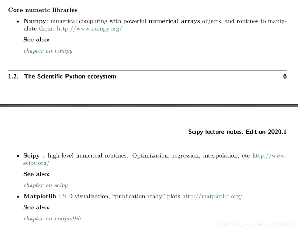 這三個第三方庫: NumPy, SciPy, Matplotlib 有何不同? 根據官網的 Scipy Lecture Notes 2020 版: NumPy 主要是提供對數組(array) 或矩陣(matrix)的指令 SciPy 則提供較上層的科學計算的函數: 最佳化(求極大極小), 求零根, 統計, 傅立葉變換等 SciPy 的基本內容大項: 特殊函數、積分、最佳化、訊號處理、統計等等
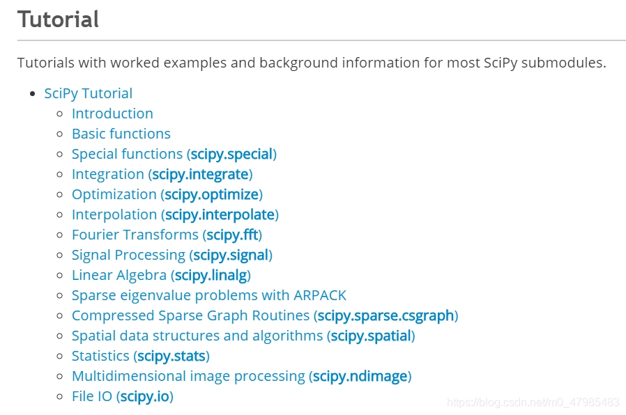
Matplotlib 則支持繪圖方面, Matplotlib.pyplot 是提供跟 Matlab 繪圖指令接近的繪圖函式庫 Ref: Scipy Lecture Notes: http://scipy-lectures.org/ link … 也可以參考許多博客的說明: 例如 csdn上的 Ref: 简述Python的Numpy,SciPy和Pandas,Matplotlib的区别, https://blog.csdn.net/ctrigger/article/details/92666676 link
Ref: 這裡有很具體的指令用法, 用在線性代數課程上: 陳擎文教學網:python解線性代數, https://acupun.site/lecture/linearAlgebra/index.htm link
Python, Numpy, SciPy 的安裝或線上使用
安裝Python 請參考本人的另一篇 從turtle海龜動畫 學習 Python - 高中彈性課程系列 2 安裝 Python, 線上執行 Python 安裝Python 那節 (本教材獲得國立高雄師範大學111學年度高教深耕計畫優良教材獎勵, 核撥獎金14500元)
Python安裝之後並沒有 NumPy, SciPy, Pandas 這些程式庫, 他們是額外加裝在 Python 上的程式庫 (目前仍是開源且免費), 在 Windows 下, 打開 “命令提示字元” 的視窗, (注意, 當下的路徑可能要在Python的資料夾下), 輸入
>> pip install numpy >> pip install scipy
或是使用 Anaconda, 安裝好之後, 最重要的程式庫都已裝好, Anaconda + Jupyter Notebook 會自動安裝好所需的科學計算或大數據的程式庫 (or Anaconda + Spyder or Anaconda + PyCharm 等),
或是使用 VSCode, 安裝好之後, 重要的程式庫可以當下搜尋外掛擴充.
線上使用可以用 Google Colab, 也會自動安裝好所需的科學計算或大數據的程式庫.
注意事項:
Python 的 list 之 slice(切片) 不會與原 list 連動 np.array() 的 slice 會與原 np.array 連動 特別注意 Python 的所有資料的容器(例如 list) 下標是從 0 開始, 與 C 語言相同(Matlab則是從1開始)
剛學 Python 較容易感到混淆的, 就是那些指令是本來就有的, 那些是從外部第三方庫引入的
以下提到 “Python 的 原生 $\dots$”, 指的是一安裝好就有的功能、模組、物件或指令等,
A. 本來就有(原生)指令
又分,
A.1. 打開IDLE就可以馬上用的指令(開箱即用)
可以下 dir(‘builtins’) 查看內建的指令, 發現跟下面官網的 Built-in Functions列表不太一樣
>>> dir('builtins')
['__add__', '__class__', '__contains__', '__delattr__', '__dir__', '__doc__', '__eq__', '__format__', '__ge__', '__getattribute__', '__getitem__', '__getnewargs__', '__gt__', '__hash__', '__init__', '__init_subclass__', '__iter__', '__le__', '__len__', '__lt__', '__mod__', '__mul__', '__ne__', '__new__', '__reduce__', '__reduce_ex__', '__repr__', '__rmod__', '__rmul__', '__setattr__', '__sizeof__', '__str__', '__subclasshook__', 'capitalize', 'casefold', 'center', 'count', 'encode', 'endswith', 'expandtabs', 'find', 'format', 'format_map', 'index', 'isalnum', 'isalpha', 'isascii', 'isdecimal', 'isdigit', 'isidentifier', 'islower', 'isnumeric', 'isprintable', 'isspace', 'istitle', 'isupper', 'join', 'ljust', 'lower', 'lstrip', 'maketrans', 'partition', 'replace', 'rfind', 'rindex', 'rjust', 'rpartition', 'rsplit', 'rstrip', 'split', 'splitlines', 'startswith', 'strip', 'swapcase', 'title', 'translate', 'upper', 'zfill']
以下是官網的 Built-in Functions列表, 下面有連結處
Built-in Functions: abs() delattr() hash() memoryview() set() all() dict() help() min() setattr() any() dir() hex() next() slice() ascii() divmod() id() object() sorted() bin() enumerate() input() oct() staticmethod() bool() eval() int() open() str() breakpoint() exec() isinstance() ord() sum() bytearray() filter() issubclass() pow() super() bytes() float() iter() print() tuple() callable() format() len() property() type() chr() frozenset() list() range() vars() classmethod() getattr() locals() repr() zip() compile() globals() map() reversed() import() complex() hasattr() max() round() 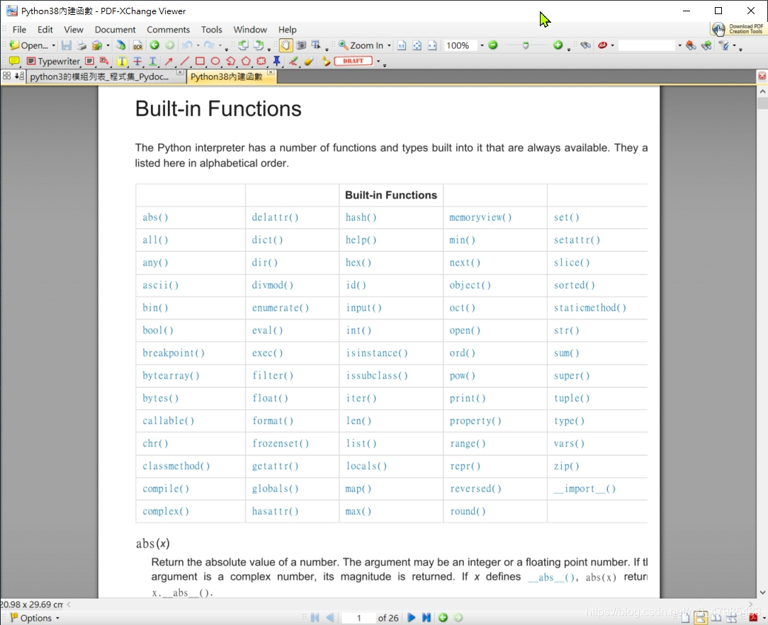
例如 abs() 就是取絕對值,,,
ref: 官網的 Built-in Functions列表 : https://docs.python.org/3/library/functions.html link
另外, 以及各內建 class 的方法, 例如 list 物件的方法, 例如 list.sort() 等, 都是開箱即用
A.2. 要先載入需要之內建模組, 例如 math, turtle 等模組需先用 import 載入才能用的指令
還有些是要載入自動安裝好的模組, 例如 求最大公因數, 可以用math.gcd(a,b) 需要先載入 math module 先下 import math 再下 math.gcd(a,b)
Python 才會認得並執行.
A.2.1 內建 數學函數與內建的 math 模組 的數學函數
內建_數學函數: abs(), comlex(), max(), min(), pow(), round(), sorted(), sum(),
內建的math 模組的數學函數: sin(), cos(), atan(),,,,fmod(), ceil(), floor(), fabs(),factorial(), exp(), gcd(), pow(x,y), log10(), sqrt(),fsum(), math.gamma(), math.pi, math.e, math.inf ( =float(‘inf’) ), math.nan ( =float(‘nan’))
ref: 內建的math 模組的數學函數: https://docs.python.org/3/library/math.html link
>>> import math >>> dir(math) [‘doc’, ‘loader’, ‘name’, ‘package’, ‘spec’, ‘acos’, ‘acosh’, ‘asin’, ‘asinh’, ‘atan’, ‘atan2’, ‘atanh’, ‘ceil’, ‘comb’, ‘copysign’, ‘cos’, ‘cosh’, ‘degrees’, ‘dist’, ‘e’, ‘erf’, ‘erfc’, ‘exp’, ‘expm1’, ‘fabs’, ‘factorial’, ‘floor’, ‘fmod’, ‘frexp’, ‘fsum’, ‘gamma’, ‘gcd’, ‘hypot’, ‘inf’, ‘isclose’, ‘isfinite’, ‘isinf’, ‘isnan’, ‘isqrt’, ‘ldexp’, ‘lgamma’, ‘log’, ‘log10’, ‘log1p’, ‘log2’, ‘modf’, ‘nan’, ‘perm’, ‘pi’, ‘pow’, ‘prod’, ‘radians’, ‘remainder’, ‘sin’, ‘sinh’, ‘sqrt’, ‘tan’, ‘tanh’, ‘tau’, ‘trunc’]
Ref Python 中有數學指令的模組或程式庫: 用 Python+SciPy+SymPy 執行微積分計算 1 link 部分參考自 陳擎文教學網, python求解數學式(高中數學,大學數學,工程數學,微積分)
- 以下可以等進階時再細看
A.2.2 查看有那些內建的模組 help(__builtins__)
要從 Windows 開始程式集 處選取, 例如 /python38/Module Docs 才看的到, 其實內容是放在安裝在硬碟的檔案, 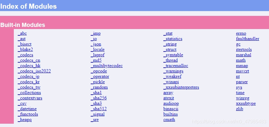 或是下
或是下 >>>help(__builtins__) 也可以
B. 需從外部安裝所謂”第三方程式庫”的指令
就是非原生的程式庫, 需要另外加裝, 例如 numpy, scipy 等以及它們的物件跟指令. 例如, 如果是 Windows 作業系統下, 需要先打開 cmd(命令提示字元), 下 pip install numpy 才算安裝好 在 IDLE 內還要下 import numpy 才能開始使用 numpy 的指令
B.1 查看已經安裝的所有模組, 包括外部模組 help('modules')
如果查看已經安裝的所有模組, 包括外部模組, 可以在 IDLE下 help('modules') 查看已經安裝的所有模組, 會顯示內建的跟已安裝的第三方程式庫,
>>> help('modules')

Please wait a moment while I gather a list of all available modules...

FactorList_Lai      autocomplete        html                runpy
__future__          autocomplete_w      http                runscript
__main__            autoexpand          hyperparser         sched
_abc                base64              idle                scipy
_ast                bdb                 idle_test           scrolledlist
_asyncio            binascii            idlelib             search
_bisect             binhex              imaplib             searchbase
_blake2             bisect              imghdr              searchengine
_bootlocale         browser             imp                 secrets
_bz2                builtins            importlib           select
_codecs             bz2                 inspect             selectors
_codecs_cn          cProfile            io                  setuptools
_codecs_hk          caesarCipher        iomenu              shelve
_codecs_iso2022     calendar            ipaddress           shlex
_codecs_jp          calltip             isympy              shutil
_codecs_kr          calltip_w           itertools           sidebar
_codecs_tw          cgi                 json                signal
_collections        cgitb               keyword             site
_collections_abc    chunk               kiwisolver          six
_compat_pickle      cmath               lib2to3             smtpd
_compression        cmd                 linecache           smtplib
_contextvars        code                locale              sndhdr
_csv                codecontext         logging             socket
_ctypes             codecs              lzma                socketserver
_ctypes_test        codeop              macosx              sqlite3
_datetime           collections         mailbox             squeezer
_decimal            colorizer           mailcap             sre_compile
_dummy_thread       colorsys            mainmenu            sre_constants
_elementtree        compileall          marshal             sre_parse
_functools          concurrent          math                ssl
_hashlib            config              matplotlib          stackviewer
_heapq              config_key          mimetypes           stat
_imp                configdialog        mmap                statistics
_io                 configparser        modulefinder        statusbar
_json               contextlib          mpmath              string
_locale             contextvars         msilib              stringprep
_lsprof             copy                msvcrt              struct
_lzma               copyreg             multicall           subprocess
_markupbase         crypt               multiprocessing     sunau
_md5                csv                 netrc               symbol
_msi                ctypes              nntplib             sympy
_multibytecodec     curses              nt                  symtable
_multiprocessing    cycler              ntpath              sys
_opcode             dataclasses         nturl2path          sysconfig
_operator           datetime            numbers             tabnanny
_osx_support        dateutil            numpy               tarfile
_overlapped         dbm                 opcode              telnetlib
_pickle             debugger            operator            tempfile
_py_abc             debugger_r          optparse            test
_pydecimal          debugobj            os                  textview
_pyio               debugobj_r          outwin              textwrap
_queue              decimal             pandas              this
_random             delegator           parenmatch          threading
_sha1               difflib             parser              time
_sha256             dis                 pathbrowser         timeForVectorMethodFactor
_sha3               distutils           pathlib             timeit
_sha512             doctest             pdb                 tkinter
_signal             dummy_threading     percolator          token
_sitebuiltins       dynoption           pickle              tokenize
_socket             easy_install        pickletools         tooltip
_sqlite3            editor              pip                 trace
_sre                email               pipes               traceback
_ssl                encodings           pkg_resources       tracemalloc
_stat               ensurepip           pkgutil             tree
_statistics         enum                platform            tty
_string             errno               plistlib            turtle
_strptime           ex1_Sum_n_Squre_3_Python_style poplib              turtledemo
_struct             ex3_check           posixpath           types
_symtable           ex4_checkRandom     pprint              typing
_testbuffer         ex5_checkRandomList profile             undo
_testcapi           faulthandler        pstats              unicodedata
_testconsole        filecmp             pty                 unittest
_testimportmultiple fileinput           py_compile          urllib
_testmultiphase     filelist            pyclbr              uu
_thread             fnmatch             pydoc               uuid
_threading_local    format              pydoc_data          venv
_tkinter            formatter           pyexpat             warnings
_tracemalloc        fractions           pylab               wave
_warnings           ftplib              pyparse             weakref
_weakref            functools           pyparsing           webbrowser
_weakrefset         gc                  pyperclip           window
_winapi             genericpath         pyshell             winreg
_xxsubinterpreters  getopt              pytz                winsound
abc                 getpass             query               wsgiref
aifc                gettext             queue               xdrlib
antigravity         glob                quopri              xml
argparse            grep                random              xmlrpc
array               gzip                re                  xxsubtype
ast                 hashlib             redirector          zipapp
asynchat            heapq               replace             zipfile
asyncio             help                reprlib             zipimport
asyncore            help_about          rlcompleter         zlib
atexit              history             rpc                 zoomheight
audioop             hmac                run                 zzdummy

Enter any module name to get more help.  Or, type "modules spam" to search
for modules whose name or summary contain the string "spam".
- 以上可以等進階時再細看
- 以下可以等進階時再細看
C. 內部指令與第三方程式庫之指令常有同名之情形, 或是不同之第三方程式庫指令會有同名之情形, 在使用時要小心
指令同名, 可能用法不同, 所以要小心! 例如 Python 有原生的 random 模組, 而 NumPy 模組的 numpy.random 也有很多類似的指令.
所以很多資料都建議, 在載入第三方程式庫時盡量不要用 from math import * 此種載入方式, 可以直接使用指令, 例如 gcd(100,25)
盡量用 import math 的方式 此種載入方式, 指令前需加一個模組名及點語法, 例如 math.gcd(100,25) 如此就可以知道, gcd()是來自於 math 模組, 如果其他模組也有 gcd(), 就不會混淆.
細節等以後再提
D. 粗略查看某個模組的所有方法或指令
可以在用 import 載入該模組之後, 使用 dir查詢 例如以下可以列出內建之 turtle 模組的所有指令 詳細的用法仍需查 Pyhton 官網的說明 https://docs.python.org/3/library/turtle.html
>>> import turtle
>>> dir(turtle)
['Canvas', 'Pen', 'RawPen', 'RawTurtle', 'Screen', 'ScrolledCanvas', 'Shape', 'TK', 'TNavigator', 'TPen', 'Tbuffer', 'Terminator', 'Turtle', 'TurtleGraphicsError', 'TurtleScreen', 'TurtleScreenBase', 'Vec2D', '_CFG', '_LANGUAGE', '_Root', '_Screen', '_TurtleImage', '__all__', '__builtins__', '__cached__', '__doc__', '__file__', '__forwardmethods', '__func_body', '__loader__', '__methodDict', '__methods', '__name__', '__package__', '__spec__', '__stringBody', '_alias_list', '_make_global_funcs', '_screen_docrevise', '_tg_classes', '_tg_screen_functions', '_tg_turtle_functions', '_tg_utilities', '_turtle_docrevise', '_ver', 'addshape', 'back', 'backward', 'begin_fill', 'begin_poly', 'bgcolor', 'bgpic', 'bk', 'bye', 'circle', 'clear', 'clearscreen', 'clearstamp', 'clearstamps', 'clone', 'color', 'colormode', 'config_dict', 'deepcopy', 'degrees', 'delay', 'distance', 'done', 'dot', 'down', 'end_fill', 'end_poly', 'exitonclick', 'fd', 'fillcolor', 'filling', 'forward', 'get_poly', 'get_shapepoly', 'getcanvas', 'getmethparlist', 'getpen', 'getscreen', 'getshapes', 'getturtle', 'goto', 'heading', 'hideturtle', 'home', 'ht', 'inspect', 'isdown', 'isfile', 'isvisible', 'join', 'left', 'listen', 'lt', 'mainloop', 'math', 'mode', 'numinput', 'onclick', 'ondrag', 'onkey', 'onkeypress', 'onkeyrelease', 'onrelease', 'onscreenclick', 'ontimer', 'pd', 'pen', 'pencolor', 'pendown', 'pensize', 'penup', 'pos', 'position', 'pu', 'radians', 'read_docstrings', 'readconfig', 'register_shape', 'reset', 'resetscreen', 'resizemode', 'right', 'rt', 'screensize', 'seth', 'setheading', 'setpos', 'setposition', 'settiltangle', 'setundobuffer', 'setup', 'setworldcoordinates', 'setx', 'sety', 'shape', 'shapesize', 'shapetransform', 'shearfactor', 'showturtle', 'simpledialog', 'speed', 'split', 'st', 'stamp', 'sys', 'textinput', 'tilt', 'tiltangle', 'time', 'title', 'towards', 'tracer', 'turtles', 'turtlesize', 'types', 'undo', 'undobufferentries', 'up', 'update', 'width', 'window_height', 'window_width', 'write', 'write_docstringdict', 'xcor', 'ycor']
如果想查NumPy 模組的所有指令, 一樣用 import 載入之後, 使用 dir查詢 指令長達 93行, 詳細的用法仍需查 Numpy 官網的說明或手冊
>>> import numpy
>>> dir(numpy)
['ALLOW_THREADS', 'AxisError', 'BUFSIZE', 'CLIP', 'ComplexWarning', 'DataSource', 'ERR_CALL',
'ERR_DEFAULT', 'ERR_IGNORE', 'ERR_LOG', 'ERR_PRINT', 'ERR_RAISE', 'ERR_WARN',
'FLOATING_POINT_SUPPORT', 'FPE_DIVIDEBYZERO', 'FPE_INVALID', 'FPE_OVERFLOW',
 'FPE_UNDERFLOW', 'False_', 'Inf', 'Infinity', 'MAXDIMS', 'MAY_SHARE_BOUNDS',
 'MAY_SHARE_EXACT', 'MachAr', 'ModuleDeprecationWarning', 'NAN', 'NINF', 'NZERO', 'NaN', 'PINF',
 'PZERO', 'RAISE', 'RankWarning', 'SHIFT_DIVIDEBYZERO', 'SHIFT_INVALID', 'SHIFT_OVERFLOW',
  'SHIFT_UNDERFLOW', 'ScalarType', 'Tester', 'TooHardError', 'True_', 'UFUNC_BUFSIZE_DEFAULT',
 'UFUNC_PYVALS_NAME', 'VisibleDeprecationWarning', 'WRAP', '_NoValue', '_UFUNC_API',
 '__NUMPY_SETUP__', '__all__', '__builtins__', '__cached__', '__config__', '__dir__', '__doc__', '__file__',
 '__getattr__', '__git_revision__', '__loader__', '__name__', '__package__', '__path__', '__spec__',
 '__version__', '_add_newdoc_ufunc', '_distributor_init', '_globals', '_mat', '_pytesttester', 'abs', 'absolute',
'absolute_import', 'add', 'add
- 以上可以等進階時再細看
Reference
LU 分解 的現成指令, 只有在 scipy.linalg 與 sympy 有看到, numpy.linalg 則沒有, scipy.linalg 與 sympy 兩者都有, cholesky, qr, svd. scipy.linalg 多 lu, shur 等 – Numpy linalg 最新列表: https://numpy.org/devdocs/reference/routines.linalg.html link – SciPy linalg 最新列表: https://docs.scipy.org/doc/scipy/reference/linalg.html#scipy.linalg link
(如果想知道Pythn更基礎的部分, 例如 list串列, 函數如何定義, random 隨機數之產生等等, 可以參考本人另一篇: 從turtle海龜動畫 學習 Python - 高中彈性課程系列 3 烏龜繪圖 所需之Python基礎 https://blog.csdn.net/m0_47985483/article/details/109522858 link
我是透過 Python 的 turtle 模組, 切入 Python 的使用, turtle 模組有較豐富的說明文件, 也可以觀摩源程式碼, 感謝 Python 的 turtle 模組的開發人員! (用 Python 的 turtle 模組探索數學, 可以參考本人的正在寫的另一篇: 從turtle海龜動畫學習Python-高中彈性課程1 link.
官網的 Built-in Functions列表 : https://docs.python.org/3/library/functions.html link
內建的math 模組的數學函數: https://docs.python.org/3/library/math.html link
Scipy Lecture Notes: http://scipy-lectures.org/ link
也可以參考許多博客的說明: 例如 csdn上的, 简述Python的Numpy,SciPy和Pandas,Matplotlib的区别, https://blog.csdn.net/ctrigger/article/details/92666676 link
推薦: 這裡有很具體的指令用法, 用在線性代數課程上: Python 中有數學指令的模組或程式庫: 陳擎文教學網, python求解數學式(高中數學,大學數學,工程數學,微積分)https://acupun.site/lecture/python_math/index.htm#chp5 link
如果想立即參考 Python+ Numpy用在線性代數課程上的指令之例子, 可先看以下陳擎文這份網頁, (我提醒你官網的文件建議盡量用 numpy.array( , ), 不要用 numpy.matrix, 陳擎文這份網頁有很多用 matrix ) Ref: 陳擎文教學網這裡有很具體的指令用法, 用在線性代數課程上: 陳擎文教學網:python解線性代數, https://acupun.site/lecture/linearAlgebra/index.htm link
- Thesaurus of Mathematical Languages, or MATLAB synonymous commands in Python/NumPy 列出 Matlab, Python, R, Octave等, 相對應的指令, 有 pdf檔. Copyright ©2006,2008 Vidar Bronken Gundersen, http://mathesaurus.sf.net/ link
- NumPy for Matlab users 列出 Matlab, Python 相對應的指令. https://numpy.org/doc/stable/user/numpy-for-matlab-users.html link
- SciPy: Tentative_NumPy_Tutorial https://scipy.github.io/old-wiki/pages/Tentative_NumPy_Tutorial link
SciPy: Numpy_Example_List 很有用的指令列表, 很長按字母順序排, 都有例子, 非常棒! https://scipy.github.io/old-wiki/pages/Numpy_Example_List.html link
- numpy.linalg 與 scipy.linalg 會有不少相同的 array 指令, 兩者都有的指令, 該用那個? https://docs.scipy.org/doc/scipy/reference/tutorial/linalg.html#scipy-linalg-vs-numpy-linalg 以上官網這裡提到, numpy.linalg有的, scipy.linalg都有, 且更進階更快! scipy.linalg contains all the functions in numpy.linalg. plus some other more advanced ones not contained in numpy.linalg. Another advantage of using scipy.linalg over numpy.linalg is that it is always compiled with BLAS/LAPACK support, while for numpy this is optional. Therefore, the scipy version might be faster depending on how numpy was installed. Therefore, unless you don’t want to add scipy as a dependency to your numpy program, use scipy.linalg instead of numpy.linalg. link
- numpy.matrix vs 2-D numpy.ndarray 該用那個? numpy 有 ndarray 類, 也有 matrix矩陣類, matrix矩陣類操作更直觀且指令與matlab更接近, 但是官網建議盡量用 numpy.array( ,,, ), https://docs.scipy.org/doc/scipy/reference/tutorial/linalg.html#scipy-linalg-vs-numpy-linalg numpy.matrix vs 2-D numpy.ndarray “The classes that represent matrices, and basic operations, such as matrix multiplications and transpose are a part of numpy. For convenience, we summarize the differences between numpy.matrix and numpy.ndarray here. numpy.matrix is matrix class that has a more convenient interface than numpy.ndarray for matrix operations. This class supports, for example, MATLAB-like creation syntax via the semicolon, has matrix multiplication as default for the * operator, and contains I and T members that serve as shortcuts for inverse and transpose: Despite its convenience, the use of the numpy.matrix class is discouraged, since it adds nothing that cannot be accomplished with 2-D numpy.ndarray objects, and may lead to a confusion of which class is being used. For example, the above code can be rewritten as: ,,,,,,” link
Sorting how to, https://github.com/python/cpython/blob/3.8/Doc/howto/sorting.rst link
- Clever B Moler, Numerical computing with Matlab.
- 劉正君, Matlab 科學計算與可視化仿真, 電子工業.
- 張若愚, Pyhton 科學計算.
猿媛之家, Python 程序員面試筆試寶典, 機械工業出版,
- Python函數的返回值與嵌套函數 - 每日頭條, 函數基本解釋, 閉包解釋清楚簡單 https://kknews.cc/zh-tw/code/ngopzeg.html link
20250406
用 Python+Numpy+scipy 執行矩陣計算 2 scipy.linalg 官網完整列表
scipy.linalg 官網完整列表
https://docs.scipy.org/doc/scipy/reference/linalg.html#scipy.linalg
Linear algebra (scipy.linalg) Linear algebra functions.
See also
numpy.linalg for more linear algebra functions. Note that although scipy.linalg imports most of them, identically named functions from scipy.linalg may offer more or slightly differing functionality. ==numpy.linalg 與 scipy.linalg 有很多同名的函數, 通常 scipy.linalg 的同名函數會提供較豐富的功能==.
Basics
| 指令 | 說明 |
|---|---|
| inv(a[, overwrite_a, check_finite]) | Compute the inverse of a matrix. |
| solve(a, b[, sym_pos, lower, overwrite_a, …]) | Solves the linear equation set a * x = b for the unknown x for square a matrix. |
| solve_banded(l_and_u, ab, b[, overwrite_ab, …]) | Solve the equation a x = b for x, assuming a is banded matrix. |
| solveh_banded(ab, b[, overwrite_ab, …]) | Solve equation a x = b. |
| solve_circulant(c, b[, singular, tol, …]) | Solve C x = b for x, where C is a circulant matrix. |
| solve_triangular(a, b[, trans, lower, …]) | Solve the equation a x = b for x, assuming a is a triangular matrix. |
| solve_toeplitz(c_or_cr, b[, check_finite]) | Solve a Toeplitz system using Levinson Recursion |
| matmul_toeplitz(c_or_cr, x[, check_finite, …]) | Efficient Toeplitz Matrix-Matrix Multiplication using FFT |
| det(a[, overwrite_a, check_finite]) | Compute the determinant of a matrix |
| norm(a[, ord, axis, keepdims, check_finite]) | Matrix or vector norm. |
| lstsq(a, b[, cond, overwrite_a, …]) | Compute least-squares solution to equation Ax = b. |
| pinv(a[, atol, rtol, return_rank, …]) | Compute the (Moore-Penrose) pseudo-inverse of a matrix. |
| pinv2(a[, cond, rcond, return_rank, …]) | Compute the (Moore-Penrose) pseudo-inverse of a matrix. |
| pinvh(a[, atol, rtol, lower, return_rank, …]) | Compute the (Moore-Penrose) pseudo-inverse of a Hermitian matrix. |
| kron(a, b) | Kronecker product. |
| khatri_rao(a, b) | Khatri-rao product |
| tril(m[, k]) | Make a copy of a matrix with elements above the kth diagonal zeroed. |
| triu(m[, k]) | Make a copy of a matrix with elements below the kth diagonal zeroed. |
| orthogonal_procrustes(A, B[, check_finite]) | Compute the matrix solution of the orthogonal Procrustes problem. |
| matrix_balance(A[, permute, scale, …]) | Compute a diagonal similarity transformation for row/column balancing. |
| subspace_angles(A, B) | Compute the subspace angles between two matrices. |
| bandwidth(a) | Return the lower and upper bandwidth of a 2D numeric array. |
| issymmetric(a[, atol, rtol]) | Check if a square 2D array is symmetric. |
| ishermitian(a[, atol, rtol]) | Check if a square 2D array is Hermitian. |
| LinAlgError | Generic Python-exception-derived object raised by linalg functions. |
| LinAlgWarning | The warning emitted when a linear algebra related operation is close to fail conditions of the algorithm or loss of accuracy is expected. |
Eigenvalue Problems
指令 | 說明 :——– | :—– eig(a[, b, left, right, overwrite_a, …]) | Solve an ordinary or generalized eigenvalue problem of a square matrix. eigvals(a[, b, overwrite_a, check_finite, …]) | Compute eigenvalues from an ordinary or generalized eigenvalue problem. eigh(a[, b, lower, eigvals_only, …]) | Solve a standard or generalized eigenvalue problem for a complex Hermitian or real symmetric matrix. eigvalsh(a[, b, lower, overwrite_a, …]) | Solves a standard or generalized eigenvalue problem for a complex Hermitian or real symmetric matrix. eig_banded(a_band[, lower, eigvals_only, …]) | Solve real symmetric or complex Hermitian band matrix eigenvalue problem. eigvals_banded(a_band[, lower, …]) | Solve real symmetric or complex Hermitian band matrix eigenvalue problem. eigh_tridiagonal(d, e[, eigvals_only, …]) | Solve eigenvalue problem for a real symmetric tridiagonal matrix. eigvalsh_tridiagonal(d, e[, select, …]) | Solve eigenvalue problem for a real symmetric tridiagonal matrix.
Decompositions
指令 | 說明 :——– | :—– lu(a[, permute_l, overwrite_a, check_finite]) | Compute pivoted LU decomposition of a matrix. lu_factor(a[, overwrite_a, check_finite]) | Compute pivoted LU decomposition of a matrix. lu_solve(lu_and_piv, b[, trans, …]) | Solve an equation system, a x = b, given the LU factorization of a svd(a[, full_matrices, compute_uv, …]) | Singular Value Decomposition. svdvals(a[, overwrite_a, check_finite]) | Compute singular values of a matrix. diagsvd(s, M, N) | Construct the sigma matrix in SVD from singular values and size M, N. orth(A[, rcond]) | Construct an orthonormal basis for the range of A using SVD null_space(A[, rcond]) | Construct an orthonormal basis for the null space of A using SVD ldl(A[, lower, hermitian, overwrite_a, …]) | Computes the LDLt or Bunch-Kaufman factorization of a symmetric/ hermitian matrix. cholesky(a[, lower, overwrite_a, check_finite]) | Compute the Cholesky decomposition of a matrix. cholesky_banded(ab[, overwrite_ab, lower, …]) | Cholesky decompose a banded Hermitian positive-definite matrix cho_factor(a[, lower, overwrite_a, check_finite]) | Compute the Cholesky decomposition of a matrix, to use in cho_solve cho_solve(c_and_lower, b[, overwrite_b, …]) | Solve the linear equations A x = b, given the Cholesky factorization of A. cho_solve_banded(cb_and_lower, b[, …]) | Solve the linear equations A x = b, given the Cholesky factorization of the banded Hermitian A. polar(a[, side]) | Compute the polar decomposition. qr(a[, overwrite_a, lwork, mode, pivoting, …]) | Compute QR decomposition of a matrix. qr_multiply(a, c[, mode, pivoting, …]) | Calculate the QR decomposition and multiply Q with a matrix. qr_update(Q, R, u, v[, overwrite_qruv, …]) | Rank-k QR update qr_delete(Q, R, k, int p=1[, which, …]) | QR downdate on row or column deletions qr_insert(Q, R, u, k[, which, rcond, …]) | QR update on row or column insertions rq(a[, overwrite_a, lwork, mode, check_finite]) | Compute RQ decomposition of a matrix. qz(A, B[, output, lwork, sort, overwrite_a, …]) | QZ decomposition for generalized eigenvalues of a pair of matrices. ordqz(A, B[, sort, output, overwrite_a, …]) | QZ decomposition for a pair of matrices with reordering. schur(a[, output, lwork, overwrite_a, sort, …]) | Compute Schur decomposition of a matrix. rsf2csf(T, Z[, check_finite]) | Convert real Schur form to complex Schur form. hessenberg(a[, calc_q, overwrite_a, …]) | Compute Hessenberg form of a matrix. cdf2rdf(w, v) | Converts complex eigenvalues w and eigenvectors v to real eigenvalues in a block diagonal form wr and the associated real eigenvectors vr, such that. cossin(X[, p, q, separate, swap_sign, …]) | Compute the cosine-sine (CS) decomposition of an orthogonal/unitary matrix.
See also
scipy.linalg.interpolative – Interpolative matrix decompositions https://docs.scipy.org/doc/scipy/reference/linalg.interpolative.html#module-scipy.linalg.interpolative link
## Matrix Functions
| 指令 | 說明 |
|---|---|
| expm(A) | Compute the matrix exponential using Pade approximation. |
| logm(A[, disp]) | Compute matrix logarithm. |
| cosm(A) | Compute the matrix cosine. |
| sinm(A) | Compute the matrix sine. |
| tanm(A) | Compute the matrix tangent. |
| coshm(A) | Compute the hyperbolic matrix cosine. |
| sinhm(A) | Compute the hyperbolic matrix sine. |
| tanhm(A) | Compute the hyperbolic matrix tangent. |
| signm(A[, disp]) | Matrix sign function. |
| sqrtm(A[, disp, blocksize]) | Matrix square root. |
| funm(A, func[, disp]) | Evaluate a matrix function specified by a callable. |
| expm_frechet(A, E[, method, compute_expm, …]) | Frechet derivative of the matrix exponential of A in the direction E. |
| expm_cond(A[, check_finite]) | Relative condition number of the matrix exponential in the Frobenius norm. |
| fractional_matrix_power(A, t) | Compute the fractional power of a matrix. |
Matrix Equation Solvers
指令 | 說明 :——– | :—– solve_sylvester(a, b, q) | Computes a solution (X) to the Sylvester equation . solve_continuous_are(a, b, q, r[, e, s, …]) | Solves the continuous-time algebraic Riccati equation (CARE). solve_discrete_are(a, b, q, r[, e, s, balanced]) | Solves the discrete-time algebraic Riccati equation (DARE). solve_continuous_lyapunov(a, q) | Solves the continuous Lyapunov equation . solve_discrete_lyapunov(a, q[, method]) | Solves the discrete Lyapunov equation .
Sketches and Random Projections
指令 | 說明 :—–| :—— clarkson_woodruff_transform(input_matrix, …) | Applies a Clarkson-Woodruff Transform/sketch to the input matrix.
Special Matrices
指令 | 說明 :—–| :—— block_diag(*arrs) | Create a block diagonal matrix from provided arrays. circulant( c ) | Construct a circulant matrix. companion(a) | Create a companion matrix. convolution_matrix(a, n[, mode]) | Construct a convolution matrix. dft(n[, scale]) | Discrete Fourier transform matrix. fiedler(a) | Returns a symmetric Fiedler matrix fiedler_companion(a) | Returns a Fiedler companion matrix hadamard(n[, dtype]) | Construct an Hadamard matrix. hankel(c[, r]) | Construct a Hankel matrix. helmert(n[, full]) | Create an Helmert matrix of order n. hilbert(n) | Create a Hilbert matrix of order n. invhilbert(n[, exact]) | Compute the inverse of the Hilbert matrix of order n. leslie(f, s) | Create a Leslie matrix. pascal(n[, kind, exact]) | Returns the n x n Pascal matrix. invpascal(n[, kind, exact]) | Returns the inverse of the n x n Pascal matrix. toeplitz(c[, r]) | Construct a Toeplitz matrix. tri(N[, M, k, dtype]) | Construct (N, M) matrix filled with ones at and below the kth diagonal.
Low-level routines
指令 | 說明 :—–| :—— get_blas_funcs(names[, arrays, dtype, ilp64]) | Return available BLAS function objects from names. get_lapack_funcs(names[, arrays, dtype, ilp64]) | Return available LAPACK function objects from names. find_best_blas_type([arrays, dtype]) | Find best-matching BLAS/LAPACK type.
See also
scipy.linalg.blas – Low-level BLAS functions https://docs.scipy.org/doc/scipy/reference/linalg.blas.html#module-scipy.linalg.blas link
scipy.linalg.lapack – Low-level LAPACK functions https://docs.scipy.org/doc/scipy/reference/linalg.lapack.html#module-scipy.linalg.lapack link
scipy.linalg.cython_blas – Low-level BLAS functions for Cython https://docs.scipy.org/doc/scipy/reference/linalg.cython_blas.html#module-scipy.linalg.cython_blas link
scipy.linalg.cython_lapack – Low-level LAPACK functions for Cython https://docs.scipy.org/doc/scipy/reference/linalg.cython_lapack.html#module-scipy.linalg.cython_lapack link
Reference
LU 分解 的現成指令, 只有在 scipy.linalg 與 sympy 有看到,numpy.linalg 則沒有, 兩者都有, cholesky, qr, svd. scipy.linalg 多 lu, shur 等 – Numpy linalg 最新列表: https://numpy.org/devdocs/reference/routines.linalg.html link – SciPy linalg 最新列表: https://docs.scipy.org/doc/scipy/reference/linalg.html#scipy.linalg link
Numpy Mathematical functions Numpy 的數學函數列表 https://numpy.org/devdocs/reference/routines.math.html link
[矩阵的QR分解系列一] 施密特(Schmidt)正交规范化, https://blog.csdn.net/honyniu/article/details/109959777 link.
用 Python+Numpy+scipy 執行 Matlab 的矩陣計算 3 產生 numpy 的 數組, 矩陣點乘 等
以下直接以例子講解
以下例子會同步將原生 list 與 numpy 模組 的 np.array() 兩種作比較, 可能讀者剛讀會有點混淆, 只要注意, 有 np. 開頭的就是numpy 模組 的 np.array() , 沒有就是指 原生 list.
Python 的 原生 list(串列 or列表) 是最常用的放資料的容器, 用 [ ] 包住就是
Python 的 原生 list: [a,b,c,d,$\dots$]
>>> [1,2,3,4,5]
[1, 2, 3, 4, 5]
>>> type([1,2,3,4,5])
<class 'list'>
Python 原生最簡單產生數列的方式: range(start, end, stride) ( Matlab: start:stride:end)
range(1,6) 會產生 1,2,3,4,5
>>> range(1,6)
range(1, 6)
>>> type(range(10))
<class 'range'>
他是一個 跌代器 iterator, 為了提高效能, 不會印出來, 要看他的內容, 要用 for loop print 印出來
>>> for i in range(1,6):
  print(i)
1
2
3
4
5
>>> for i in range(1,6,2):
  print(i)
1
3
5
如果要由大到小 用 令 b>a, range(b,a,-1) 會得到 b,b-1,,,a+1 例如 range(10,5,-1)
>>> for i in range(10,5,-1):
  print(i)
10
9
8
7
6
NumPy 數組 np.array 最簡單產生 numpy 數列的方式: np.arange(start, end, stride) (Matlab: start:stride:end)
產生 a 到 (b-1) 間格 間格 gap, 之 等分點, 可以用以下指令, 指定間格寬度為 gap np.arange(a, b, gap) 就是 np.arange(start, end, stride) arrange 是 array range 的意思, 是 numpy 的指令, 初學容易跟原生的 range 混淆
>>> np.arange(1,6)
array([1, 2, 3, 4, 5])

>>> np.arange(1,6,2)
array([1, 3, 5])
>>> type(np.arange(1,6))
<class 'numpy.ndarray'>
# 反轉
>>> np.arange(10,5,-1)
array([10,  9,  8,  7,  6])
- 以下可以等進階時再細看
Python 的 原生 list 做 copy 要小心
Python 的 原生 list 可以放 list在裡面, 可以是較複雜的, 例如 以下, a 串列的元素有純量, 有 list, 也有 dict (字典),
>>> a = [1,2,3,[4,5,6],'abc',{'a':1,'b':2,'c':3}]
>>> a
[1, 2, 3, [4, 5, 6], 'abc', {'a': 1, 'b': 2, 'c': 3}]
註: 因為Python 的 原生 list 可以放一層一層的資料容器在內, 在copy 時會出現不預期的狀況, 後面介紹深拷貝跟淺拷貝, 有點繁瑣, 建議第一次閱讀, 可以跳過. 如果只是要拷貝某個 aList 內容, 不想跟原來的 aList 會有連動, 就用
import copy aDeepCopy=aList.copy.deepcopy()
執行深複製, 全部(各層)不連動, 避免產生不預期的狀況.
以上可以等進階時再細看
list 的 擷取元素與切片 (indexing 與 slicing)
>>> aList = [1,2,3,4,5]
>>> aList
[1, 2, 3, 4, 5]
取用 aList 的其中一個元素, 我們稱為 indexing, 取用第 index 個元素
特別注意 Python 的所有資料的容器(例如 list) 下標是從 0 開始 ( Python, C, JavaScript 下標是從 0 開始 Matlab, R 下標是從 1 開始 )
>>> aList[0]
1
>>> aList[1]
2
取用 aList 的其中一段元素, 我們稱為 slicing (slice 切片)
所謂 slicing 語法, 是指 n:m 語法
>>> aList[1:3]
[2, 3]
>>> b = aList[1:3]
>>> b
[2, 3]
b 是 aList 的 slice, a 改變, 不會影響 b ( Python 的 list 之 slice 不會連動) (注意: np.array()的 slice 會連動)
>>> aList[1]=22
>>> aList
[1, 22, 3, 4, 5]
>>> b
[2, 3]
Python 的 list 不能用 真假值或整數 list 取切片 但是 np.array 可以用 真假值或整數 之 np.array 或 lis 取切片
請參考後面 fancy indexing: np.array 的切片可以用 真假值之 list 或整數 之 list 或 np.array 做下標集, 提取內容, 但不連動
>>> aList
[0, 1, 2, 3, 4, 5, 6, 7, 8, 9]
>>> aList[[0,2,4]]
Traceback (most recent call last):
  File "<pyshell#76>", line 1, in <module>
    aList[[0,2,4]]
TypeError: list indices must be integers or slices, not list
- 以下可以等進階時再細看
list 複製
Python 深淺拷貝, 只差在第二層以上 當 list 中含有 list 時, 深淺拷貝才會有差別
*aCopy1=aList[:] 淺複製, 只有第一層不連動
aCopy1=aList[:] 當 aList 改變 其中一個純量元素 時, aCopy 不會連動
>>> aList = [1,22,3,4,5]
>>> aCopy1 = aList[:]
>>> aCopy1
[1, 22, 3, 4, 5]
>>> aCopy1[0]=2
>>> aCopy1
[2, 22, 3, 4, 5]
>>> aList
[1, 22, 3, 4, 5]
對於 aList 是 list 含有 list 時
>>> aList = [1,2,3,4,[1,2,3]]
>>> aCopy = alist[:]
>>> aCopy
[1, 2, 3, 4, [1, 2, 3]]
>>> aList[4][0]=11
>>> aList
[1, 2, 3, 4, [11, 2, 3]]
>>> aCopy
[1, 2, 3, 4, [11, 2, 3]]
aCopy=aList.copy() 淺複製, 只有第一層不連動
aCopy=aList.copy() 當 aList 改變 其中一個純量元素 時, aCopy 不會連動
>>> aList
[1, 22, 3, 4, 5]
>>> aCopy=aList.copy()
>>> aCopy
[1, 22, 3, 4, 5]
>>> aCopy is aList
False
>>> aCopy == aList
True
>>> aCopy[0]=2
>>> aCopy
[2, 22, 3, 4, 5]
>>> aList
[1, 22, 3, 4, 5]
當 list 中含有 list 時, 如果只改變 list 中的 list 的一個元素 時, 淺拷貝還是會連動 當 aList 改變 list 中的 list 的一個元素 時, aCopy 也跟著改了
>>> aList = [1,22,3,4,[1,2,3]]
>>> aList
[1, 22, 3, 4, [1, 2, 3]]
>>> aCopy=aList.copy()
>>> aCopy
[1, 22, 3, 4, [1, 2, 3]]
>>> aList[0]=2
>>> aList
[2, 22, 3, 4, [1, 2, 3]]
>>> aCopy
[1, 22, 3, 4, [1, 2, 3]]
# 當 aList 改變  list 中的 list 的一個元素 時, aCopy 也跟著改了
>>> aList[4][1]=0
>>> aList
[2, 22, 3, 4, [1, 0, 3]]
>>> aCopy
[1, 22, 3, 4, [1, 0, 3]]
>>> aList[4] == aCopy[4]
True
>>> aList[4] is aCopy[4]
True
>>> aList[0] is aCopy[0]
True
>>> aList is aCopy
False
# 當 aList 改變 其中一個純量元素 時, aCopy 不會改
>>> aList[0]=3
>>> aList
[3, 22, 3, 4, [1, 0, 3]]
>>> aCopy
[2, 22, 3, 4, [1, 0, 3]]
當 aList 改變 list 中的 整個 list 時, 淺拷貝不連動 如果把 list 中的 list, 整條換掉, 似乎指向 list 中的該 list 的位址就改變了, 就把 aList[4] 與 aCopy[4] 的關聯脫鉤了! ( 如果只是更改 aList[4][1], 則 aList[4] 與 aCopy[4] 仍是同位址)
>>> aList[4]=[11,0,33]
>>> aList
[3, 22, 3, 4, [11, 0, 33]]
>>> aCopy
[2, 22, 3, 4, [1, 0, 3]]
>>> aList[4][1]=2
>>> aList
[3, 22, 3, 4, [11, 2, 33]]
>>> aCopy
[2, 22, 3, 4, [1, 0, 3]]
>>> aList[4] is aCopy[4]
False
以上可以等進階時再細看
深複製, 全部(各層)不連動
import copy aDeepCopy=copy.deepcopy(aList)
>>> import copy
>>> aDeepCopy=aList.copy.deepcopy()
Traceback (most recent call last):
  File "<pyshell#39>", line 1, in <module>
    aDeepCopy=aList.copy.deepcopy()
AttributeError: 'builtin_function_or_method' object has no attribute 'deepcopy'
>>> aDeepCopy=copy.deepcopy(aList)
>>> aDeepCopy
[1, 22, 3, 4, 5]
>>> aDeepCopy is aList
False
>>> aDeepCopy == aList
True
即使 aList 是一個 list 中含有 list, aDeepCopy是深複製得來的, 它還是, 各層都不會與 aList 連動
>>> aList = [1,2,3,4,[1,2,3]]
>>> aDeepCopy = copy.deepcopy(aList)
>>> aDeepCopy
[1, 2, 3, 4, [1, 2, 3]]
>>> aList[4][0] = 11
>>> aList
[1, 2, 3, 4, [11, 2, 3]]
>>> aDeepCopy
[1, 2, 3, 4, [1, 2, 3]]
複製但連動, 完全一樣
用等號 aListRef = aList, 其實是得到完全一樣
>>> aListRef = aList
>>> aListRef
[1, 22, 3, 4, 5]
>>> aListRef == aList
True
>>> aListRef is aList
True
產生 numpy 的 數組: np.array(), (Matlab: [1,2,3; 4,5,6])
對照: 劉正君, 3.4
>>> import numpy as np
>>> A = np.array([[1,2,3],[4,5,6]]);A
array([[1, 2, 3],
       [4, 5, 6]])
>>> B = np.arange(11,17);B
array([11, 12, 13, 14, 15, 16])
>>> B.reshape(3,2)
array([[11, 12],
       [13, 14],
       [15, 16]])
產生 numpy 的 數組: 各類特殊矩陣: 零矩陣、都是1的矩陣、 單位矩陣(對角線為1之矩陣)、 取用對角線矩陣、 上三角矩陣
ref: 劉正君, 3.6. 3
zeros filled array 零矩陣 (Matlab: zeros(3,5))
>>> a = np.zeros(5)
>>> a
array([0., 0., 0.,>>> a1 = np.zeros([5,5])
>>> a1
array([[0., 0., 0., 0., 0.],
       [0., 0., 0., 0., 0.],
       [0., 0., 0., 0., 0.],
       [0., 0., 0., 0., 0.],
       [0., 0., 0., 0., 0.]]) 0., 0.])
# 注意, 維度用 [5,5] 包住
>>> a1 = np.ones(5,5);a1
Traceback (most recent call last):
  File "<pyshell#5>", line 1, in <module>
    a1 = np.ones(5,5);a1
  File "C:\Users\user\AppData\Local\Programs\Python\Python38-32\lib\site-packages\numpy\core\numeric.py", line 207, in ones
    a = empty(shape, dtype, order)
TypeError: data type not understood
ones filled array 1矩陣 (Matlab: ones(3,5))
>>> b = np.ones(5)
>>> b
array([1., 1., 1., 1., 1.])
>>> b1 = np.ones([5,5])
>>> b1
array([[1., 1., 1., 1., 1.],
       [1., 1., 1., 1., 1.],
       [1., 1., 1., 1., 1.],
       [1., 1., 1., 1., 1.],
       [1., 1., 1., 1., 1.]])
any number filled array 任意數字填滿矩陣 (Matlab: ones(3,5)*9 )
>>> b2 = b1*3
>>> b2
array([[3., 3., 3., 3., 3.],
       [3., 3., 3., 3., 3.],
       [3., 3., 3., 3., 3.],
       [3., 3., 3., 3., 3.],
       [3., 3., 3., 3., 3.]])
identity array 單位矩陣(對角線矩陣) (Matlab: eye(3))
>>> c = np.eye(4)
>>> c
array([[1., 0., 0., 0.],
       [0., 1., 0., 0.],
       [0., 0., 1., 0.],
       [0., 0., 0., 1.]])
>>> c1 = np.identity(4)
>>> c1
array([[1., 0., 0., 0.],
       [0., 1., 0., 0.],
       [0., 0., 1., 0.],
       [0., 0., 0., 1.]])
給定 np.array a 取用a 的對角線 (Matlab: diag(a), diag(a,0))
>>> a
array([[1, 2, 3],
       [4, 5, 6],
       [7, 8, 9]])
>>> a_diag = np.diag(a)
>>> a_diag
array([1, 5, 9])
>>> a_diag2d = a_diag*np.eye(3)
>>> a_diag2d
array([[1., 0., 0.],
       [0., 5., 0.],
       [0., 0., 9.]])
隨機數組 (Matlab: rand(3,4))
>>> a_rand = np.random.rand(3,4)
>>> a_rand
array([[0.65543729, 0.32649166, 0.21621299, 0.58931067],
       [0.7932652 , 0.35415987, 0.83885435, 0.02375679],
       [0.01526737, 0.95740181, 0.36366563, 0.66846968]])
改變形狀 np.reshape()、 np.resize() (Matlab: reshape(1:6,3,2))
注意: 使用 reshape()時, 原array沒改變!
>>> B=np.array([11, 12, 13, 14, 15, 16])
>>> B
array([11, 12, 13, 14, 15, 16])
# 將 B reshape() 後的 array指定給 B1
>>> B1 = B.reshape(2,3)
>>> B1
array([[11, 12, 13],
       [14, 15, 16]])
# B 原 array 沒改變
>>> B
array([11, 12, 13, 14, 15, 16])
注意 A.reshape 後指定給另一個名稱, 例如 A_reform, A 與 A_reform 會連動,
>>> A = np.arange(1,11)
>>> A
array([ 1,  2,  3,  4,  5,  6,  7,  8,  9, 10])
>>> A.reshape(2,5)
array([[ 1,  2,  3,  4,  5],
       [ 6,  7,  8,  9, 10]])
>>> A
array([ 1,  2,  3,  4,  5,  6,  7,  8,  9, 10])
>>> A_reform=A.reshape(2,5)
>>> A_reform
array([[ 1,  2,  3,  4,  5],
       [ 6,  7,  8,  9, 10]])
>>> A_reform[1,2]
8
>>> A_reform[1,2]=18
>>> A_reform
array([[ 1,  2,  3,  4,  5],
       [ 6,  7, 18,  9, 10]])
>>> A
array([ 1,  2,  3,  4,  5,  6,  7, 18,  9, 10])
注意: 使用 resize()時, 原array會改變!
>>> B2 = np.resize(B,(3,2))
>>> B2
array([[11, 12],
       [13, 14],
       [15, 16]])
>>> B
array([[11, 12],
       [13, 14],
       [15, 16]])
用 B2 = B.resize(3,2)會出錯
>>> B2 = B.resize(3,2)
>>> B2
>>> B2[0]
Traceback (most recent call last):
  File "<pyshell#46>", line 1, in <module>
    B2[0]
TypeError: 'NoneType' object is not subscriptable
np.array()的元素可以是那些?
基本上就是整數、浮點數、複數、字串等
>>> np.typeDict.values()
dict_values([<class 'numpy.bool_'>, <class 'numpy.bool_'>, <class 'numpy.int8'>, <class 'numpy.int8'>, <class 'numpy.int8'>, <class 'numpy.uint8'>, <class 'numpy.uint8'>, <class 'numpy.uint8'>, <class 'numpy.int16'>, <class 'numpy.int16'>, <class 'numpy.int16'>, <class 'numpy.uint16'>, <class 'numpy.uint16'>, <class 'numpy.uint16'>, <class 'numpy.intc'>, <class 'numpy.intc'>, <class 'numpy.uint32'>, <class 'numpy.uintc'>, <class 'numpy.uintc'>, <class 'numpy.intc'>, <class 'numpy.intc'>, <class 'numpy.uintc'>, <class 'numpy.uintc'>, <class 'numpy.int32'>, <class 'numpy.int32'>, <class 'numpy.int32'>, <class 'numpy.uint32'>, <class 'numpy.uint32'>, <class 'numpy.int64'>, <class 'numpy.int64'>, <class 'numpy.int64'>, <class 'numpy.uint64'>, <class 'numpy.uint64'>, <class 'numpy.uint64'>, <class 'numpy.float16'>, <class 'numpy.float16'>, <class 'numpy.float16'>, <class 'numpy.float32'>, <class 'numpy.float32'>, <class 'numpy.float64'>, <class 'numpy.float64'>, <class 'numpy.float64'>, <class 'numpy.longdouble'>, <class 'numpy.longdouble'>, <class 'numpy.longdouble'>, <class 'numpy.complex128'>, <class 'numpy.complex64'>, <class 'numpy.complex64'>, <class 'numpy.complex128'>, <class 'numpy.complex128'>, <class 'numpy.complex128'>, <class 'numpy.clongdouble'>, <class 'numpy.clongdouble'>, <class 'numpy.clongdouble'>, <class 'numpy.object_'>, <class 'numpy.object_'>, <class 'numpy.bytes_'>, <class 'numpy.bytes_'>, <class 'numpy.str_'>, <class 'numpy.str_'>, <class 'numpy.str_'>, <class 'numpy.void'>, <class 'numpy.void'>, <class 'numpy.void'>, <class 'numpy.datetime64'>, <class 'numpy.datetime64'>, <class 'numpy.timedelta64'>, <class 'numpy.timedelta64'>, <class 'numpy.bool_'>, <class 'numpy.bool_'>, <class 'numpy.bool_'>, <class 'numpy.int32'>, <class 'numpy.int32'>, <class 'numpy.int32'>, <class 'numpy.uint32'>, <class 'numpy.uintc'>, <class 'numpy.uint32'>, <class 'numpy.float16'>, <class 'numpy.float16'>, <class 'numpy.float16'>, <class 'numpy.float32'>, <class 'numpy.float32'>, <class 'numpy.float32'>, <class 'numpy.float64'>, <class 'numpy.float64'>, <class 'numpy.float64'>, <class 'numpy.complex64'>, <class 'numpy.complex64'>, <class 'numpy.complex64'>, <class 'numpy.complex128'>, <class 'numpy.complex128'>, <class 'numpy.complex128'>, <class 'numpy.object_'>, <class 'numpy.object_'>, <class 'numpy.bytes_'>, <class 'numpy.bytes_'>, <class 'numpy.str_'>, <class 'numpy.str_'>, <class 'numpy.void'>, <class 'numpy.void'>, <class 'numpy.datetime64'>, <class 'numpy.datetime64'>, <class 'numpy.datetime64'>, <class 'numpy.timedelta64'>, <class 'numpy.timedelta64'>, <class 'numpy.timedelta64'>, <class 'numpy.uint32'>, <class 'numpy.int64'>, <class 'numpy.int64'>, <class 'numpy.int64'>, <class 'numpy.uint64'>, <class 'numpy.uint64'>, <class 'numpy.uint64'>, <class 'numpy.int16'>, <class 'numpy.int16'>, <class 'numpy.int16'>, <class 'numpy.uint16'>, <class 'numpy.uint16'>, <class 'numpy.uint16'>, <class 'numpy.int8'>, <class 'numpy.int8'>, <class 'numpy.int8'>, <class 'numpy.uint8'>, <class 'numpy.uint8'>, <class 'numpy.uint8'>, <class 'numpy.complex128'>, <class 'numpy.intc'>, <class 'numpy.uintc'>, <class 'numpy.float32'>, <class 'numpy.complex64'>, <class 'numpy.complex64'>, <class 'numpy.float64'>, <class 'numpy.intc'>, <class 'numpy.uintc'>, <class 'numpy.int32'>, <class 'numpy.longdouble'>, <class 'numpy.clongdouble'>, <class 'numpy.clongdouble'>, <class 'numpy.bool_'>, <class 'numpy.bytes_'>, <class 'numpy.bytes_'>, <class 'numpy.str_'>, <class 'numpy.object_'>, <class 'numpy.str_'>, <class 'numpy.int32'>, <class 'numpy.float64'>, <class 'numpy.complex128'>, <class 'numpy.bool_'>, <class 'numpy.object_'>, <class 'numpy.str_'>, <class 'numpy.bytes_'>, <class 'numpy.bytes_'>])
如果元素是 list, 或是 np.array 的類型,也可以
>>> a=np.array(['a','b',[1,2]])
>>> a
array(['a', 'b', list([1, 2])], dtype=object)
>>> a=np.array(['a','b',np.array([1,2])])
>>> a
array(['a', 'b', array([1, 2])], dtype=object)
>>> a[0]
'a'
>>> a[2]
array([1, 2])
為何不用 Python 的 原生 list 來執行類似數組的操作?
Ans:
- NumPy 的 array 是用 C 的 知名線性代數工具庫 去計算, 而 list 的效能並沒有用 C 優化,
- NumPy 的 array 允許用真假值(布林值)或整數 之 list 或 真假值(布林值)或整數 之 np.array 做下標集, 提取內容, 但 list 無此功能
有關上面 2. 的測試: 產生一個 Python 的 原生 list
# 產生一個 Python 的 原生 list
>>> aList = [0,1,2,3,4,5]
>>> aList
[0, 1, 2, 3, 4, 5]
# 定義一個真假值(布林值) list
>>> booleanIndex = [ True, False, True, False, True, False]
# 用真假值(布林值)做下標集, 提取
# 出現錯誤訊息, 顯示, list 的 下標集只能用單一整數或是 slices 切片(用 n:m 語法)
>>> aList[booleanIndex]
Traceback (most recent call last):
  File "<pyshell#3>", line 1, in <module>
    aList[booleanIndex]
TypeError: list indices must be integers or slices, not list
產生一個 np 的 array, 用跟上面一樣的真假值(布林值) list: booleanIndex 去提取內容, 發現可以!
>>> import numpy as np
>>> aArray = np.array([0,1,2,3,4,5])
>>> aArray
array([0, 1, 2, 3, 4, 5])
>>> aArray[booleanIndex]
array([0, 2, 4])
>>>
請參考後面 fancy indexing: np.array 的切片可以用 真假值之 list 或整數 之 list 或 np.array 做下標集, 提取內容, 但不連動
A 的長寬高 A.shape(), A 的元素個數 A.size (Matlab: size(A), length(A))
array (或matrix) 常需要維度的訊息
>>> A.shape
(2, 3)
>>> np.shape(A)
(2, 3)
>>> len(A)
2
>>> B.shape
(6,)
>>> B1.shape
(3, 2)
>>> B2.shape
(2, 3)

>>> A.size
6
>>> np.size(A)
6
A 的維度有幾維 A.ndim (Matlab: ndims(A))
以下Array 有3維 在操作線性代數時, 有時會需要知道該數組的維度有幾維
>>> aArray = np.array([[[1,2,3],[4,5,6]],[[7,8,9],[10,11,12]]])
>>> aArray
array([[[ 1,  2,  3],
        [ 4,  5,  6]],

       [[ 7,  8,  9],
        [10, 11, 12]]])
>>> aArray.ndim
3
此時 A 與 B1的維度相合, 就可以進行矩陣相乘
矩陣相乘
- 在 Matlab 中是用 A * B1,
- 在 numpy中用 numpy.dot(A, B1), 或是
- numpy.matmul(A,B1)
>>> np.dot(A,B1)
array([[ 82,  88],
       [199, 214]])
>>> np.matmul(A,B1)
array([[ 82,  88],
       [199, 214]])
矩陣點乘
- 在 Matlab 中是用 A .* B
- 在 numpy中用 A*B
>>> B2=B.reshape(2,3)
>>> B2
array([[11, 12, 13],
       [14, 15, 16]])
>>> A*B2
array([[11, 24, 39],
       [56, 75, 96]])
>>> np.multiply(A,B2)
array([[11, 24, 39],
       [56, 75, 96]])
矩陣點除
- 在 Matlab 中是用 A ./ B
- 在 numpy中用 A/B
>>> A/B2
array([[0.09090909, 0.16666667, 0.23076923],
     [0.28571429, 0.33333333, 0.375     ]])
矩陣複製
np 中最常出錯的是對一個array 做 copy 的動作 ref: Scipy lecture notes, Edition 2020.1: sec 4.1.6 copy and view **ref: 何敏煌, Python 程式設計實務, sec 6.3.5: a is b **
如果直接用 A1= A
則得到一個完全一樣的 A, 只是多一個別名叫 A1 而已, 此時你改變 A1, 就等於改變A, A 與 A1 都指向同一個位址
>>> A1 = A
>>> A1 is A
True
>>> A.shape
(2, 3)
>>> A1.shape
(2, 3)
>>> A1.shape=(3,2)
>>> A1.shape
(3, 2)
>>> A.shape
(3, 2)
>>> A
array([[1, 2],
     [3, 4],
     [5, 6]])
>>> A1
array([[1, 2],
     [3, 4],
     [5, 6]])
>>> id(A)
60451360
>>> id(A1)
60451360
切片是 view 會連動
view 是(淺層)拷貝 (shallow) copy 取 slicing 就是 view 當 S 是 A 的 slice, 改變 S, 也會改變 A, 會連動
>>> A
array([[1, 2],
     [3, 4],
     [5, 6]])
>>> S = A[:,1]
>>> S
array([2, 4, 6])
>>> S[:] = 10
>>> S
array([10, 10, 10])
>>> A
array([[ 1, 10],
     [ 3, 10],
     [ 5, 10]])
copy(), id()
copy 是(深層)拷貝 (deep) copy D = A.copy(), 則D 的資料與 A 一樣, 但是, 位址不同, 改變D, 與 A 無關! ```python
D = A.copy() D array([[ 1, 10], [ 3, 10], [ 5, 10]]) D is A False D[0,:]=9 D array([[ 9, 9], [ 3, 10], [ 5, 10]]) A array([[ 1, 10], [ 3, 10], [ 5, 10]])
id(A) 60451360 id(D) 206144320 ```
fancy indexing: np.array 的切片可以用 真假值之 list 或整數 之 list 或 np.array 做下標集, 提取內容, 但不連動
NumPy 的 array 允許用真假值(布林值)或整數 之 list 或 真假值(布林值)或整數 之 np.array 做下標集, 提取內容(但 list 無此功能), 與原來的 array 不連動, scipy lecture notes 稱此為 fancy indexing.
ref: Scipy lecture notes, Edition 2020.1: sec4.1.7 Fancy indexing
以下用 整數 之 list 取切片, 不連動
>>> import numpy as np
>>> aArray = np.array([1,2,3,4,5])
>>> aArray
array([1, 2, 3, 4, 5])
>>> aArray[[0,1,4]]
array([1, 2, 5])
>>> bArray = aArray[[0,1,4]]
>>> bArray
array([1, 2, 5])
>>> aArray[0]=22
>>> aArray
array([22,  2,  3,  4,  5])
>>> bArray
array([1, 2, 5])
>>> bArray[0]=11
>>> bArray
array([11,  2,  5])
>>> aArray
array([22,  2,  3,  4,  5])
>>> arrayIndex = np.array([1,2,4])
>>> arrayIndex
array([1, 2, 4])
>>> bArray = aArray[arrayIndex]
>>> bArray
array([2, 3, 5])
以下用 整數 之 np.array 取切片, 不連動
>>> arrayIndex = np.array([0,1,4])
>>> arrayIndex
array([0, 1, 4])
>>> bArray = aArray[arrayIndex]
>>> bArray
array([22,  2,  5])
>>> aArray[0]=222
>>> aArray
array([222,   2,   3,   4,   5])
>>> bArray
array([22,  2,  5])
NumPy 的 速查簡表
Ref: 以下我們參考: Python Numpy全世界最長基礎教程最適合小白學習 還詳細很全速拿, https://twgreatdaily.com/AhWyTG8BMH2_cNUgWU4g.html link.
一、數組方法
創建數組:arange()創建一維數組;array()創建一維或多維數組,其參數是類似於數組的對象,如列表等
創建數組:np.zeros((2,3)),或者np.ones((2,3)),參數是一個元組分別表示行數和列數
對應元素相乘,a * b,得到一個新的矩陣,形狀要一致;但是允許a是向量而b是矩陣,a的列數必須等於b的列數,a與每個行向量點乘
- / 與 * 的運算規則相同。
數學上定義的矩陣乘法 np.dot(a, b)。如果形狀不匹配會報錯;但是允許允許a和b都是向量,返回兩個向量的內積。只要有一個參數不是向量,就應用矩陣乘法。
(PS:總之就是,向量很特殊,在運算中可以自由轉置而不會出錯,運算的返回值如果維度為1,也一律用行向量[]表示)
讀取數組元素:如a[0],a[0,0]
數組變形:如b=a.reshape(2,3,4)將得到原數組變為234的三維數組後的數組;或是a.shape=(2,3,4)或a.resize(2,3,4)直接改變數組a的形狀
數組組合:水平組合hstack((a,b))或concatenate((a,b),axis=1);垂直組合vstack((a,b))或concatenate((a,b),axis=0);深度組合dstack((a,b))
數組分割(與數組組合相反):分別有hsplit,vsplit,dsplit,split(split與concatenate相對應)
將np數組變為py列表:a.tolist()
數組排序(小到大):列排列np.msort(a),行排列np.sort(a),np.argsort(a)排序後返回下標
複數排序:np.sort_complex(a)按先實部後虛部排序
數組的插入:np.searchsorted(a,b)將b插入原有序數組a,並返回插入元素的索引值
類型轉換:如a.astype(int),np的數據類型比py豐富,且每種類型都有轉換方法
條件查找,返回滿足條件的數組元素的索引值:np.where(條件)
條件查找,返回下標:np.argwhere(條件)
>>> A
array([ 1,  4,  7, 10])
>>> np.argwhere(A==7)
array([[2]], dtype=int64)
>>> np.where(A==7)
(array([2], dtype=int64),)
>>> np.where(A%2==0)
(array([1, 3], dtype=int64),)
>>> np.argwhere(A%2==0)
array([[1],
       [3]], dtype=int64)
條件查找,返回滿足條件的數組元素:np.extract([條件],a)
根據b中元素作為索引,查找a中對應元素:np.take(a,b)一維
數組中最小最大元素的索引:np.argmin(a),np.argmax(a)
多個數組的對應位置上元素大小的比較:np.maximum(a,b,c,…..)返回每個索引位置上的最大值,np.minimum(…….)相反
將a中元素都置為b:a.fill(b)
每個數組元素的指數:np.exp(a)
生成等差行向量:如np.linspace(1,6,10)則得到1到6之間的均勻分布,總共返回10個數
求余:np.mod(a,n)相當於a%n,np.fmod(a,n)仍為求余且餘數的正負由a決定
計算平均值:np.mean(a)
計算最大值:amax(a, axis=None, out=None, keepdims=False) 。Return the maximum of an array or maximum along an axis.
計算加權平均值:np.average(a,b),其中b是權重
計算數組的極差:np.pth(a)=max(a)-min(a)
計算方差(總體方差):np.var(a)
標準差:np.std(a)
算術平方根,a為浮點數類型:np.sqrt(a)
對數:np.log(a)
修剪數組,將數組中小於x的數均換為x,大於y的數均換為y:a.clip(x,y)
所有數組元素乘積:a.prod()
數組元素的累積乘積:a.cumprod()
數組元素的符號:np.sign(a),返回數組中各元素的正負符號,用1和-1表示
數組元素分類:np.piecewise(a,[條件],[返回值]),分段給定取值,根據判斷條件給元素分類,並返回設定的返回值。
判斷兩數組是否相等: np.array_equal(a,b)
判斷數組元素是否為實數: np.isreal(a)
去除數組中首尾為0的元素:np.trim_zeros(a)
對浮點數取整,但不改變浮點數類型:np.rint(a)
二、數組屬性
1.獲取數組每一維度的大小:a.shape
2.獲取數組維度:a.ndim
3.元素個數:a.size
4.數組元素在內存中的字節數:a.itemsize
5.數組字節數:a.nbytes==a.size*a.itemsize
6.數組元素覆蓋:a.flat=1,則a中數組元素都被1覆蓋
7.數組轉置:a.T
不能求逆、求協方差、跡等,不適用於複雜科學計算,可以將array轉換成matrix。
三、矩陣方法
==np.mat(『…』) 官網已建議不要使用== 創建矩陣:np.mat(『…』)通過字符串格式創建,np.mat(a)通過array數組創建,也可用matrix或bmat函數創建
創建複合矩陣:np.bmat(『A B』,』AB』),用A和B創建複合矩陣AB(字符串格式)
創建n*n維單位矩陣:np.eye(n)
矩陣的轉置:A.T
矩陣的逆矩陣:A.I
計算協方差矩陣:np.cov(x),np.cov(x,y)
計算矩陣的跡(對角線元素和):a.trace()
相關係數:np.corrcoef(x,y)
給出對角線元素:a.diagonal()
四、線性代數
估計線性模型中的係數:a=np.linalg.lstsq(x,b),有b=a*x
求方陣的逆矩陣:np.linalg.inv(A)
求廣義逆矩陣:np.linalg.pinv(A)
求矩陣的行列式:np.linalg.det(A)
解形如AX=b的線性方程組:np.linalg.solve(A,b)
求矩陣的特徵值:np.linalg.eigvals(A)
求特徵值和特徵向量:np.linalg.eig(A)
Svd分解:np.linalg.svd(A)
五、機率分布
產生二項分布的隨機數:np.random.binomial(n,p,size=…),其中n,p,size分別是每輪試驗次數、機率、輪數
產生超幾何分布隨機數:np.random.hypergeometric(n1,n2,n,size=…),其中參數意義分別是物件1總量、物件2總量、每次採樣數、試驗次數
產生N個正態分布的隨機數:np.random.normal(均值,標準差,N)
產生N個對數正態分布的隨機數:np.random.lognormal(mean,sigma,N)
六、多項式
多項式擬合:poly= np.polyfit(x,a,n),擬合點集a得到n級多項式,其中x為橫軸長度,返回多項式的係數
多項式求導函數:np.polyder(poly),返回導函數的係數
得到多項式的n階導函數:多項式.deriv(m = n)
多項式求根:np.roots(poly)
多項式在某點上的值:np.polyval(poly,x[n]),返回poly多項式在橫軸點上x[n]上的值
兩個多項式做差運算: np.polysub(a,b)
Matpoltlib簡單繪圖方法
引入簡單繪圖的包import matplotlib.pyplot as plt,最後用plt.show()顯示圖像
基本畫圖方法:plt.plot(x,y),plt.xlabel(『x』),plt.ylabel(『y』),plt.title(『…』)
子圖:plt.subplot(abc),其中abc分別表示子圖行數、列數、序號
創建繪圖組件的頂層容器:fig = plt.figure()
添加子圖:ax = fig.add_subplot(abc)
設置橫軸上的主定位器:ax.xaxis.set_major_locator(…)
繪製方圖:plt.hist(a,b),a為長方形的左橫坐標值,b為柱高
繪製散點圖:plt.scatter(x,y,c = 『..』,s = ..),c表示顏色,s表示大小
添加網格線:plt.grid(True)
添加注釋:如ax.annotate(‘x’, xy=xpoint, textcoords=’offsetpoints’,xytext=(-50, 30), arrowprops=dict(arrowstyle=”->”))
增加圖例:如plt.legend(loc=’best’, fancybox=True)
對坐標取對數:橫坐標plt.semilogx(),縱坐標plt.semilogy(),橫縱同時plt.loglog()
NumPy 與 Matlab, R, Octave 等的對照速查簡表
可以參考以下 References.
References
- Python Numpy全世界最長基礎教程最適合小白學習 還詳細很全速拿, https://twgreatdaily.com/AhWyTG8BMH2_cNUgWU4g.html link.
Python NumPy 與 Matlab, R, Octave 等的對照:
Thesaurus of Mathematical Languages, or MATLAB synonymous commands in Python/NumPy 列出 Matlab, Python, R, Octave等, 相對應的指令, 有 pdf檔. Copyright ©2006,2008 Vidar Bronken Gundersen, http://mathesaurus.sf.net/ link
NumPy for Matlab users 列出 Matlab, Python 相對應的指令. https://numpy.org/doc/stable/user/numpy-for-matlab-users.html link
用 Python+Numpy+scipy 執行矩陣計算 4 向量與矩陣運算
執行線代的例子
Ref: Clever B Moler, Numerical computing with Matlab Moler的書: Ch2 線性代數
線性聯立方程指令求解
\(Ax=B\) \(\left( \begin{array}{c c} 10 & -7 & 0 \\ -3 & 2 & 6 \\ 5 & -1 & 5 \\ \end{array} \right) \left( \begin{array}{c c} x_1 \\ x_2 \\ x_3 \\ \end{array} \right) = \left( \begin{array}{c c} b_1 \\ b_2 \\ b_3 \\ \end{array} \right)\\\) where \(A = \left( \begin{array}{c c} 10 & -7 & 0 \\ -3 & 2 & 6 \\ 5 & -1 & 5 \\ \end{array} \right)\\ x = \left( \begin{array}{c c} x_1 \\ x_2 \\ x_3 \\ \end{array} \right)\\ B= \left( \begin{array}{c c} b_1 \\ b_2 \\ b_3 \\ \end{array} \right)\)
Matalb 的指令 x=A\B
x=A\B
Python + np + scipy 的指令 x= scipy.linalg.solve(A,B)
>>> import numpy as np
>>> A=np.array([[10,-7,0],[-3,2,6],[5,-1,5]])
>>> A
array([[10, -7,  0],
       [-3,  2,  6],
       [ 5, -1,  5]])
>>> B = np.array([7,4,6])
>>> B
array([7, 4, 6])
>>> x=A\B
SyntaxError: unexpected character after line continuation character
>>> from scipy import linalg
>>> x= scipy.linalg.solve(A,B)
>>> x
array([ 0., -1.,  1.])
可以檢查解出之x 是否為解, 計算 Ax 看是否會等於 B np.dot(A,x)
>>> np.dot(A,x)
array([7., 4., 6.])
發現與 B 相等, 解為正確
Moler 的書: 2.4 排列矩陣
NumPy 排列可以用 np.random.permutation()
Python 內建的 random 模組可以用
random.shuffle() 隨機洗牌 random.sample() 隨機抽樣
>>> permu=np.random.permutation(5)
>>> permu
array([2, 0, 3, 1, 4])
>>> permu=np.random.permutation(5);permu
array([4, 0, 1, 2, 3])
>>> import random
>>> data = [1,2,3,4,5,6,7]
>>> random.shuffle(data)
>>> data
[7, 1, 3, 4, 5, 6, 2]
>>> random.sample([1,2,3,4],2)
[4, 2]
>>> random.sample([1,2,3,4],4)
[2, 4, 1, 3]
>>> random.sample([1,2,3,4,5],5)
[3, 2, 4, 5, 1]
>>> random.sample([1,2,3,4,5],5)
[1, 2, 4, 3, 5]
產生一個排列矩陣
>>> permu=random.sample(range(5),5)
>>> permu
[3, 4, 0, 1, 2]
>>> P=np.zeros((5,5));P
array([[0., 0., 0., 0., 0.],
       [0., 0., 0., 0., 0.],
       [0., 0., 0., 0., 0.],
       [0., 0., 0., 0., 0.],
       [0., 0., 0., 0., 0.]])
>>> P[0,permu[0]]=1
>>> P
array([[0., 0., 0., 1., 0.],
       [0., 0., 0., 0., 0.],
       [0., 0., 0., 0., 0.],
       [0., 0., 0., 0., 0.],
       [0., 0., 0., 0., 0.]])

>>> for i in range(5):
  P[i,permu[i]]=1


>>> P
array([[0., 0., 0., 1., 0.],
       [0., 0., 0., 0., 1.],
       [1., 0., 0., 0., 0.],
       [0., 1., 0., 0., 0.],
       [0., 0., 1., 0., 0.]])
向量(點列)之操作
Ref: 劉正君, ch3 向量與矩陣運算, Matlab 科學計算與可視化仿真, 電子工業.
產生點列 np.arange(start, end, stride) ( Matlab start:stride:end)
此指令強調切完之後的間格為 stride (預設是1). 產生 a 到 (b-1) 間格 gap, 之 等分點, 可以用以下指令, 指定間格寬度為 gap np.arange(a, b, gap) 就是 np.arange(start, end, stride) arrange 是 array range 的意思, 是 numpy 的指令, 初學容易跟原生的 range 混淆
>>> np.arange(1,6)
array([1, 2, 3, 4, 5])

>>> np.arange(1,6,2)
array([1, 3, 5])
>>> type(np.arange(1,6))
<class 'numpy.ndarray'>
# 反轉
>>> np.arange(10,5,-1)
array([10,  9,  8,  7,  6])
>>> a= np.arange(1,50,1)
>>> a
array([ 1,  2,  3,  4,  5,  6,  7,  8,  9, 10, 11, 12, 13, 14, 15, 16, 17,
       18, 19, 20, 21, 22, 23, 24, 25, 26, 27, 28, 29, 30, 31, 32, 33, 34,
       35, 36, 37, 38, 39, 40, 41, 42, 43, 44, 45, 46, 47, 48, 49])
>>> np.arange(10,0,-1)
array([10,  9,  8,  7,  6,  5,  4,  3,  2,  1])
切割成共 k 個點 np.linspace(n, m, k) ( Matlab linspace(n, m, k))
此指令強調切完之後的點數為 k. 對初學學者容易誤會, 要小心!!
為切成含頭尾等分之總共 k 個點, 有 k-1個間格, 間格長度為 (m-n)/(k-1)
a=np.linspace(0,1,11) 則切成含頭尾等分之11個點 (小心: 切10個間格,間格1/10, 含頭尾兩點總共11個點) array([0. , 0.1, 0.2, 0.3, 0.4, 0.5, 0.6, 0.7, 0.8, 0.9, 1. ])
如果下 a=np.linspace(0,1,10), 則為切9個間格, 間格1/9, 含頭尾總共10個點
array([0.        , 0.11111111, 0.22222222, 0.33333333, 0.44444444,
       0.55555556, 0.66666667, 0.77777778, 0.88888889, 1.        ])
這種結果, 很可能不是你的原意!
如果沒也指定 k, 也就是沒有指定切割成多少點, 則預設切成含頭尾共50個點 a=np.linspace(0,49) 從0到49, 預設切成等分之 含頭尾共50個點 (間格 1)
array([ 0.,  1.,  2.,  3.,  4.,  5.,  6.,  7.,  8.,  9., 10., 11., 12.,
       13., 14., 15., 16., 17., 18., 19., 20., 21., 22., 23., 24., 25.,
       26., 27., 28., 29., 30., 31., 32., 33., 34., 35., 36., 37., 38.,
       39., 40., 41., 42., 43., 44., 45., 46., 47., 48., 49.])
如果是以下, 則間格不是 1, 是 50/49 a=np.linspace(0,50)
array([ 0.        ,  1.02040816,  2.04081633,  3.06122449,  4.08163265,
        5.10204082,  6.12244898,  7.14285714,  8.16326531,  9.18367347,
       10.20408163, 11.2244898 , 12.24489796, 13.26530612, 14.28571429,
       15.30612245, 16.32653061, 17.34693878, 18.36734694, 19.3877551 ,
       20.40816327, 21.42857143, 22.44897959, 23.46938776, 24.48979592,
       25.51020408, 26.53061224, 27.55102041, 28.57142857, 29.59183673,
       30.6122449 , 31.63265306, 32.65306122, 33.67346939, 34.69387755,
       35.71428571, 36.73469388, 37.75510204, 38.7755102 , 39.79591837,
       40.81632653, 41.83673469, 42.85714286, 43.87755102, 44.89795918,
       45.91836735, 46.93877551, 47.95918367, 48.97959184, 50.        ])
如果要 0~50 間格1 等分, 可以用以下指令較順, 指定間格寬度為1 np.arange(start, end, stride) ( Matlab start:stride:end)
>>>a= np.arange(1,50,1)
array([ 1,  2,  3,  4,  5,  6,  7,  8,  9, 10, 11, 12, 13, 14, 15, 16, 17,
       18, 19, 20, 21, 22, 23, 24, 25, 26, 27, 28, 29, 30, 31, 32, 33, 34,
       35, 36, 37, 38, 39, 40, 41, 42, 43, 44, 45, 46, 47, 48, 49])
簡而言之 a=np.linspace(n, m, k), 切割 n 到 m, 為指定含頭尾總共 k 個點, 此指令強調切完之後的點數為 k (預設含頭尾共50個點). a= np.arange(n, m, s), 切割 n 到 m, 指定間格寬度為 s, np.arange(start, end, stride), 此指令強調切完之後的間格為 stride (預設是1).
>>> import numpy as np
>>> a=np.array(range(1,11))
>>> a
array([ 1,  2,  3,  4,  5,  6,  7,  8,  9, 10])
>>> a=np.linspace(1,10,10)
>>> a
array([ 1.,  2.,  3.,  4.,  5.,  6.,  7.,  8.,  9., 10.])
>>> a=np.linspace(0,1,11)
>>> a
array([0. , 0.1, 0.2, 0.3, 0.4, 0.5, 0.6, 0.7, 0.8, 0.9, 1. ])
>>> a=np.linspace(0,1,10)
>>> a
array([0.        , 0.11111111, 0.22222222, 0.33333333, 0.44444444,
       0.55555556, 0.66666667, 0.77777778, 0.88888889, 1.        ])
>>> a=np.linspace(0,49)
>>> a
array([ 0.,  1.,  2.,  3.,  4.,  5.,  6.,  7.,  8.,  9., 10., 11., 12.,
       13., 14., 15., 16., 17., 18., 19., 20., 21., 22., 23., 24., 25.,
       26., 27., 28., 29., 30., 31., 32., 33., 34., 35., 36., 37., 38.,
       39., 40., 41., 42., 43., 44., 45., 46., 47., 48., 49.])
>>> a=np.linspace(0,50)
>>> a
array([ 0.        ,  1.02040816,  2.04081633,  3.06122449,  4.08163265,
        5.10204082,  6.12244898,  7.14285714,  8.16326531,  9.18367347,
       10.20408163, 11.2244898 , 12.24489796, 13.26530612, 14.28571429,
       15.30612245, 16.32653061, 17.34693878, 18.36734694, 19.3877551 ,
       20.40816327, 21.42857143, 22.44897959, 23.46938776, 24.48979592,
       25.51020408, 26.53061224, 27.55102041, 28.57142857, 29.59183673,
       30.6122449 , 31.63265306, 32.65306122, 33.67346939, 34.69387755,
       35.71428571, 36.73469388, 37.75510204, 38.7755102 , 39.79591837,
       40.81632653, 41.83673469, 42.85714286, 43.87755102, 44.89795918,
       45.91836735, 46.93877551, 47.95918367, 48.97959184, 50.        ])
>>> 50/49
1.0204081632653061
>>> a= np.arange(1,50,1)
>>> a
array([ 1,  2,  3,  4,  5,  6,  7,  8,  9, 10, 11, 12, 13, 14, 15, 16, 17,
       18, 19, 20, 21, 22, 23, 24, 25, 26, 27, 28, 29, 30, 31, 32, 33, 34,
       35, 36, 37, 38, 39, 40, 41, 42, 43, 44, 45, 46, 47, 48, 49])
3.2.4 向量內積(矩陣點乘) np.dot(u,v), np.vdot(u,v) (Matlab dot(u,v))
>>> aArray = np.array([1,2,3,4,5])
>>> bArray = np.array([11,12,13,14,15])
>>> np.dot(aArray,bArray)
205
>>> np.vdot(aArray,bArray)
205
3.2.3 向量外積 np.cross(u,v) (Matlab cross(u,v))
只能用 3 維的向量
>>> a3dArray = np.array([1,2,3])
>>> b3dArray = np.array([11,12,13])
>>> np.cross(a3dArray,b3dArray)
array([-10,  20, -10])
3.2.6 反轉向量(或list) (Matlab: y=wrev(x))
令 b>a, arange(b,a,-1) 會得到 b,b-1,,,a+1 (令 b>a, range(b,a,-1) 會得到 b,b-1,,,a+1, 是原生的 range() )
>>> for i in range(5,1,-1):
  print(i)
5
4
3
2
>>> a= np.array([11,12,13,14,15])
>>>> np.arange(4,0,-1)
array([4, 3, 2, 1])
>>> a[np.arange(4,0,-1)]
array([15, 14, 13, 12])
原生 list 用 list.reverse() 反轉list
>>> a=[1,2,3,4,5]
>>> a.reverse()
>>> a
[5, 4, 3, 2, 1]
np.array 無此 a.reverse() 指令, (1D np.array 可以用緊接此處之後提到的 reversed(a) )
>>> a=np.array([1,2,3,4,5])
>>> a.reverse()
Traceback (most recent call last):
  File "<pyshell#75>", line 1, in <module>
    a.reverse()
AttributeError: 'numpy.ndarray' object has no attribute 'reverse'
原生 list 或 1d 的 np.array 可以用 reversed() 反轉向量
ref: 猿媛之家, Python 程序員面試筆試寶典, 機械工業出版, 2.6.8. reversed() 是內建的指令(built-in function), 可以用在 序列類 或 1d 的 np.array 都可以, reversed(a) 不會改變 a, reversed() 傳回一個迭代器 iterator, 必須用 for print才看的到內容:
>>> for i in reversed(np.array([5,4,3,2,1])):
  print(i)
1
2
3
4
5
reversed() 用在 序列類, 會傳回一個迭代器 iterator
>>> reversed([5,4,3,2,1])
<list_reverseiterator object at 0x03016E68>
>>> for i in reversed([5,4,3,2,1]):
  print(i)
1
2
3
4
5
如果是用在 2d np.array, 則只是調換 row 的次序
>>> np.array([[1,2,3],[4,5,6]])
array([[1, 2, 3],
       [4, 5, 6]])
>>> for i in reversed(np.array([[1,2,3],[4,5,6]])):
  print(i)

[4 5 6]
[1 2 3]
Ex: 寫一個可以反轉 2d np.array 的函數 Ans:
# 43鄭蕙倪 40王培瑜 36董伊真 33何宛庭 23李鈞菱 4林姵綺
# EX:寫一個可以反轉 2d np.array 的函數
import numpy as np
arr2D=np.array([[11,12,13,14],[54,55,56,57]])
reversedArr=np.flip(arr2D)
print(reversedArr)
sort 排序 list.sort(), sorted(a) (Matlab: y=wrev(x))
ref: Sorting how to, https://github.com/python/cpython/blob/3.8/Doc/howto/sorting.rst link “Python lists have a built-in list.sort() method that modifies the list in-place. There is also a sorted() built-in function that builds a new sorted list from an iterable.” 官網的 sorting how to 這篇, 講到, list.sort() 是 list 類內建的指令, sorted()則是 built-in funciton, 所有的 iterable 都可以, 所謂 iterable 氏只有順序的容器, 例如 list, tuple, dict 等, 但是只有原生的可以, 例如第三方庫的纇 np.array 後面示例不行,
a.sort() 會改變 a, 原生 list 有, np.array 也有此指令
>>> a = [3,1,5,6,4]
>>> a.sort()
>>> a
[1, 3, 4, 5, 6]
b = sorted(a) 不會改變 a, 原生 list 有, 只可用在 1d 的 np.array
>>> a = [3,1,5,6,4]
>>> b = sorted(a)
>>> a
[3, 1, 5, 6, 4]
>>> b
[1, 3, 4, 5, 6]
a.sort(), 可用在 所有維度的 np.array 但是 sorted(a) 只可用在 1d 的 np.array
>>> a = np.array([3,1,2])
>>> a.sort()
>>> a
array([1, 2, 3])
>>> a = np.array([3,1,2])
>>> b = sorted(a)
>>> a
array([3, 1, 2])
>>> b
[1, 2, 3]
2D np.array 只有 a.sort() 可以用
>>> a2D = np.array([[3,1,2],[5,4,6]])
>>> a2D
array([[3, 1, 2],
       [5, 4, 6]])
>>> a2D.sort()
>>> a2D
array([[1, 2, 3],
       [4, 5, 6]])
>>> a2D = np.array([[3,1,2],[5,4,6]])
>>> b2D = sorted(a2D)
Traceback (most recent call last):
  File "<pyshell#65>", line 1, in <module>
    b2D = sorted(a2D)
ValueError: The truth value of an array with more than one element is ambiguous. Use a.any() or a.all()
reversed(), sorted() 都是 built-in functions
>>> dir(__builtins__)
['ArithmeticError', 'AssertionError', 'AttributeError', 'BaseException', 'BlockingIOError', 'BrokenPipeError', 'BufferError', 'BytesWarning', 'ChildProcessError', 'ConnectionAbortedError', 'ConnectionError', 'ConnectionRefusedError', 'ConnectionResetError', 'DeprecationWarning', 'EOFError', 'Ellipsis', 'EnvironmentError', 'Exception', 'False', 'FileExistsError', 'FileNotFoundError', 'FloatingPointError', 'FutureWarning', 'GeneratorExit', 'IOError', 'ImportError', 'ImportWarning', 'IndentationError', 'IndexError', 'InterruptedError', 'IsADirectoryError', 'KeyError', 'KeyboardInterrupt', 'LookupError', 'MemoryError', 'ModuleNotFoundError', 'NameError', 'None', 'NotADirectoryError', 'NotImplemented', 'NotImplementedError', 'OSError', 'OverflowError', 'PendingDeprecationWarning', 'PermissionError', 'ProcessLookupError', 'RecursionError', 'ReferenceError', 'ResourceWarning', 'RuntimeError', 'RuntimeWarning', 'StopAsyncIteration', 'StopIteration', 'SyntaxError', 'SyntaxWarning', 'SystemError', 'SystemExit', 'TabError', 'TimeoutError', 'True', 'TypeError', 'UnboundLocalError', 'UnicodeDecodeError', 'UnicodeEncodeError', 'UnicodeError', 'UnicodeTranslateError', 'UnicodeWarning', 'UserWarning', 'ValueError', 'Warning', 'WindowsError', 'ZeroDivisionError', '_', '__build_class__', '__debug__', '__doc__', '__import__', '__loader__', '__name__', '__package__', '__spec__', 'abs', 'all', 'any', 'ascii', 'bin', 'bool', 'breakpoint', 'bytearray', 'bytes', 'callable', 'chr', 'classmethod', 'compile', 'complex', 'copyright', 'credits', 'delattr', 'dict', 'dir', 'divmod', 'enumerate', 'eval', 'exec', 'exit', 'filter', 'float', 'format', 'frozenset', 'getattr', 'globals', 'hasattr', 'hash', 'help', 'hex', 'id', 'input', 'int', 'isinstance', 'issubclass', 'iter', 'len', 'license', 'list', 'locals', 'map', 'max', 'memoryview', 'min', 'next', 'object', 'oct', 'open', 'ord', 'pow', 'print', 'property', 'quit', 'range', 'repr', 'reversed', 'round', 'set', 'setattr', 'slice', 'sorted', 'staticmethod', 'str', 'sum', 'super', 'tuple', 'type', 'vars', 'zip']
用 Python+Numpy+scipy 執行矩陣計算 5 函數向量化 function vectorized
之前的系列是介紹, 向量與向量, 或是 向量與矩陣, 矩陣與矩陣 的加減乘除次方, 排序等運算, 這篇我們討論 如果有一個函數 $f(x)$ 作用在整個向量或是整個矩陣 x, 會遇到的狀況.
np 的函數會自動向量化
例如以下 我們先用 x = np.arange(0,1,0.1) 產生 np 的 array: [0. , 0.1, 0.2, 0.3, 0.4, 0.5, 0.6, 0.7, 0.8, 0.9]
再用 np.sin 作用在 x=[0. , 0.1, 0.2, 0.3, 0.4, 0.5, 0.6, 0.7, 0.8, 0.9] 得到:np.sin(x)=np.sin([0. , 0.1, 0.2, 0.3, 0.4, 0.5, 0.6, 0.7, 0.8, 0.9]) 發現 $\sin(x)$ 會依序作用在每個 $[x_1, x_2,\cdots]$, 得到 $[\sin(x_1), \sin(x_2),\cdots]$,
>>> x = np.arange(0,1,0.1)
>>> x
array([0. , 0.1, 0.2, 0.3, 0.4, 0.5, 0.6, 0.7, 0.8, 0.9])
>>> np.sin(x)
array([0.        , 0.09983342, 0.19866933, 0.29552021, 0.38941834,
       0.47942554, 0.56464247, 0.64421769, 0.71735609, 0.78332691])
由此可以看出, np 的函數會自動向量化, ==可以直接作用在整批資料的每個點上==. 但是, 如果是自己定義的函數, 就沒有自動向量化的功能, 一次只能作用在一個點.
原生或 math 等 的函數要向量化需用 np.vectorize()
接續上面的例子, 我們這次改用 math 模組的 $\sin$ 函數 作用在同樣的 x = np.arange(0,1,0.1) 上, math.sin(x) 發現出現錯誤訊息:
>>> import math
>>> import numpy as np
>>> x = np.arange(0,1,0.1)
>>> x
array([0. , 0.1, 0.2, 0.3, 0.4, 0.5, 0.6, 0.7, 0.8, 0.9])
>>> math.sin(x)
Traceback (most recent call last):
  File "<pyshell#25>", line 1, in <module>
    math.sin(x)
TypeError: only size-1 arrays can be converted to Python scalars
此時我們可以用 np.vectorize() 指令, 將 math.sin 轉成向量化的函數, 重新命名為 例如: mathSinVectorize():
>>> mathSinVectorize = np.vectorize( math.sin, otypes=[np.float])
發現 mathSinVectorize() 可以向量化作用了
>>> mathSinVectorize(x)
array([0.        , 0.09983342, 0.19866933, 0.29552021, 0.38941834,
       0.47942554, 0.56464247, 0.64421769, 0.71735609, 0.78332691])
將自定義函數轉成 向量化函數
先定義一個平方函數:
def square(x):
    return x**2
再用 numpy.vectorize() 將其轉成 向量化函數
>>> import numpy as np
>>> squareVec=np.vectorize(square)
發現可以作用在 list 上了
>>> squareVec([1,2,3,4])
array([ 1,  4,  9, 16])
用 Python+Numpy+scipy 執行矩陣計算 6 矩陣特徵值等不變量計算
本篇介紹 NumPy 的 矩陣不變量求值: 例如 行列式值, 特徵值, 特徵向量等等
註: 所謂矩陣不變量, 例如 矩陣的行列式值, 特徵值, 特徵向量等, 都是矩陣的不變量, 是指 一個矩陣, 在基底變化之後, 樣貌會改變, 但是, 新的樣貌的矩陣的行列式值等, 是跟基底變化之前的矩陣的行列式值一樣的, 有這樣的性質的矩陣量, 就叫做矩陣的不變量, 除了行列式值, 特徵值, 特徵向量之外, 還有 trace, 就是 矩陣的對角線元素的和, 等等.
何謂矩陣不變量
所謂矩陣不變量, 例如 矩陣的行列式值, 特徵值, 特徵向量等, 都是矩陣的不變量, 是指 一個矩陣, 在基底變化之後, 樣貌會改變, 但是, 新的樣貌的矩陣的行列式值等, 是跟基底變化之前的矩陣的行列式值一樣的, 有這樣的性質的矩陣量, 就叫做矩陣的不變量, 除了行列式值, 特徵值, 特徵向量之外, 還有 trace, 就是 矩陣的對角線元素的和, 等等.
相對於矩陣不變量, 就是, 某些矩陣量, 在基底變化之後, 其值會改變的量, 例如, max(矩陣所有元素), 在基底變化之後, 取矩陣所有元素的最大值, 可能就改變了.
NumPy 的 矩陣不變量計算簡表
Ref: 以下我們參考: Python Numpy全世界最長基礎教程最適合小白學習 還詳細很全速拿, https://twgreatdaily.com/AhWyTG8BMH2_cNUgWU4g.html link.
四、線性代數
求矩陣的行列式:np.linalg.det(A)
求方陣的逆矩陣:np.linalg.inv(A)
求廣義逆矩陣:np.linalg.pinv(A)
解形如 $AX=b$ 的線性方程組:np.linalg.solve(A,b)
求矩陣的特徵值:np.linalg.eigvals(A)
求特徵值和特徵向量:np.linalg.eig(A)
Svd 分解:np.linalg.svd(A)
估計線性模型中的係數:a=np.linalg.lstsq(x,b),有b=a*x
求方陣的逆矩陣:np.linalg.inv(A)
有時會看到求反矩陣可以用 A.I 的指令, 這是 numpy.mat 類的指令, 目前已建議不要用了
>>>A = numpy.array([[2,3], [4,5]])

>>>A

array([2, 3])

>>>A.I

Traceback (most recent call last):
  File "<pyshell#17>", line 1, in <module>
    A.I
AttributeError: 'numpy.ndarray' object has no attribute 'I'
numpy.linalg.inv(A)

array([[-2.5,  1.5],
       [ 2. , -1. ]])
>>>B=numpy.mat(A)

>>>B

matrix([[2, 3],
        [4, 5]])
>>>B.I

matrix([[-2.5,  1.5],
        [ 2. , -1. ]])
>>> A
array([[1, 2, 3],
       [4, 5, 6],
       [7, 8, 9]])
>>> np.linalg.det(A)
0.0
>>> A = np.array([[12,2,3],[4,5,6],[7,8,9]])
>>>> A
array([[12,  2,  3],
       [ 4,  5,  6],
       [ 7,  8,  9]])
>>> np.linalg.det(A)
-33.00000000000007
>>> np.linalg.inv(A)
array([[ 0.09090909, -0.18181818,  0.09090909],
       [-0.18181818, -2.63636364,  1.81818182],
       [ 0.09090909,  2.48484848, -1.57575758]])
>>> Ainv=np.linalg.inv(A)
>>> A*Ainv
array([[  1.09090909,  -0.36363636,   0.27272727],
       [ -0.72727273, -13.18181818,  10.90909091],
       [  0.63636364,  19.87878788, -14.18181818]])
# 注意 A 與  A 的反矩陣用點乘 *, 無法成為單位矩陣!
>>> A*Ainv
array([[  1.09090909,  -0.36363636,   0.27272727],
       [ -0.72727273, -13.18181818,  10.90909091],
       [  0.63636364,  19.87878788, -14.18181818]])
# 注意 A 與  A 的反矩陣用 np.dot() 相乘, 才是矩陣乘法, 才成為單位矩陣!
>>> np.dot(Ainv,A)
array([[ 1.00000000e+00, -1.11022302e-16, -4.16333634e-17],
       [ 4.44089210e-16,  1.00000000e+00, -2.22044605e-15],
       [-2.22044605e-16,  1.77635684e-15,  1.00000000e+00]])
求轉置矩陣 A.T
>>>A.T

array([[2, 4],
       [3, 5]])
求矩陣的特徵值 np.linalg.eigvals(A)
>>> A = np.array([[1,2],[4,5]])
>>> A
array([[1, 2],
       [4, 5]])
>>> np.linalg.eig(A)
(array([-0.46410162,  6.46410162]), array([[-0.80689822, -0.34372377],
       [ 0.59069049, -0.9390708 ]]))
>>> np.linalg.eigvals(A)
array([-0.46410162,  6.46410162])
# 以下要抽出 eigenvalues, 或 eigenvectors 遇到問題!
>>> np.linalg.eigvals(A)[0]
-0.4641016151377544
>>> np.linalg.eigvals(A)[1]
6.464101615137754
>>> np.linalg.eigvals(A)[2]
Traceback (most recent call last):
  File "<pyshell#51>", line 1, in <module>
    np.linalg.eigvals(A)[2]
IndexError: index 2 is out of bounds for axis 0 with size 2
>>> np.linalg.eigvals(A)[0,1]
Traceback (most recent call last):
  File "<pyshell#52>", line 1, in <module>
    np.linalg.eigvals(A)[0,1]
IndexError: too many indices for array: array is 1-dimensional, but 2 were indexed
>>> np.linalg.eigvals(A)[0][0]
Traceback (most recent call last):
  File "<pyshell#53>", line 1, in <module>
    np.linalg.eigvals(A)[0][0]
IndexError: invalid index to scalar variable.
>>> eigvaluesA,eigenvectorsA = np.linalg.eigvals(A)
>>> eigvaluesA
-0.4641016151377544
>>> eigenvectorsA
6.464101615137754
>>> eigvaluesA1,eigvaluesA2,eigenvectorsA = np.linalg.eigvals(A)
Traceback (most recent call last):
  File "<pyshell#57>", line 1, in <module>
    eigvaluesA1,eigvaluesA2,eigenvectorsA = np.linalg.eigvals(A)
ValueError: not enough values to unpack (expected 3, got 2)
NumPy 的 矩陣不變量計算舉例
官網的 svd(A) 分解的示例,
SciPy Numpy_Example_List, https://scipy.github.io/old-wiki/pages/Numpy_Example_List.html#svd.28.29 link
>>> from numpy import *
>>> from numpy.linalg import svd
>>> A = array([[1., 3., 5.],[2., 4., 6.]]) # A is a (2x3) matrix
>>> U,sigma,V = svd(A)
>>> print U # U is a (2x2) unitary matrix
[[-0.61962948 -0.78489445]
 [-0.78489445 0.61962948]]
>>> print sigma # non-zero diagonal elements of Sigma
[ 9.52551809 0.51430058]
>>> print V # V is a (3x3) unitary matrix
[[-0.2298477 -0.52474482 -0.81964194]
 [ 0.88346102 0.24078249 -0.40189603]
 [ 0.40824829 -0.81649658 0.40824829]]
>>> Sigma = zeros_like(A) # constructing Sigma from sigma
>>> n = min(A.shape)
>>> Sigma[:n,:n] = diag(sigma)
>>> print dot(U,dot(Sigma,V)) # A = U * Sigma * V
[[ 1. 3. 5.]
 [ 2. 4. 6.]]
Reference
Python Numpy全世界最長基礎教程最適合小白學習 還詳細很全速拿, https://twgreatdaily.com/AhWyTG8BMH2_cNUgWU4g.html link.
推薦: 這裡有很具體的指令用法, 用在線性代數課程上: 陳擎文教學網:python解線性代數, https://acupun.site/lecture/linearAlgebra/index.htm link
用 Python+Numpy+scipy 執行矩陣計算 7 矩陣分解的指令
Numpy 與 Matlab 的矩陣分解的指令
| 矩陣分解的指令 | SciPy (NumPy) | Matlab | |
|---|---|---|---|
| 矩陣的條件數 | from numpy import linalg linalg.cond() (只有 numpy 的 linalg 才有, scipy 的 linalg 沒有) | cond() | |
| rank | from numpy import linalg linalg.matrix_rank() (只有 numpy 的 linalg 才有, scipy 的 linalg 沒有) | rank() | |
| LU 分解 | linalg.lu() (只有 scipy.linalg 才有) | lu() | |
| Cholesky 分解(對稱矩陣的LU分解) | linalg.cholesky() | chol() | |
| QR: 先用 Householder’s 方法將對稱矩陣分解成 tridiagonal, 再求出 eignevalues | clinalg.qr() | qr() | |
| svd 奇異值分解 | linalg.svd() | svd() | |
| Shur 分解, Shur theorem 保證 每個方陣A都 unitarily similar to 一個三角矩陣B: $B=UAU^{*}$ | linalg.shur() (只有 scipy.linalg 才有) | shur() |
==注意:== linalg.cond(a) 是 Numpy 之下的, SciPy 之下的 linalg 沒有. ==注意:== linalg.matrix_rank(a) 是 Numpy 之下的, SciPy 之下的 linalg 沒有.
>>> import numpy
>>>> from numpy import linalg
>>>> a = numpy.ones([3,3])
>>> a
array([[1., 1., 1.],
       [1., 1., 1.],
       [1., 1., 1.]])

>>> linalg.matrix_rank(a)
1
雖然 scipy 是基於 numpy 的 package, 如果整個改成用 scipy 執行上面的動作, 會看到錯誤訊息
import scipy
from scipy import linalg
a = scipy.ones([3,3])
print(a)
print(linalg.matrix_rank(a))

>>>
============= RESTART: C:/Users/user/Desktop/linalg.matrix_rank.py =============

Warning (from warnings module):
  File "C:/Users/user/Desktop/linalg.matrix_rank.py", line 12
    a = scipy.ones([3,3])
DeprecationWarning: scipy.ones is deprecated and will be removed in SciPy 2.0.0, use numpy.ones instead
[[1. 1. 1.]
 [1. 1. 1.]
 [1. 1. 1.]]
Traceback (most recent call last):
  File "C:/Users/user/Desktop/linalg.matrix_rank.py", line 16, in <module>
    print(linalg.matrix_rank(a))
AttributeError: module 'scipy.linalg' has no attribute 'matrix_rank'
錯誤或警告訊息提到, scipy.ones() 將不再使用, 請使用 numpy.ones([3,3]), 另外也提到 scipy 的 linalg 是沒有 matrix_rank 的指令!
scipy.linalg 中有關矩陣分解的指令
Decompositions :
| 指令 | 說明 |
|---|---|
| lu(a[, permute_l, overwrite_a, check_finite]) | Compute pivoted LU decomposition of a matrix. |
| lu_factor(a[, overwrite_a, check_finite]) | Compute pivoted LU decomposition of a matrix. |
| lu_solve(lu_and_piv, b[, trans, …]) | Solve an equation system, a x = b, given the LU factorization of a |
| svd(a[, full_matrices, compute_uv, …]) | Singular Value Decomposition. |
| svdvals(a[, overwrite_a, check_finite]) | Compute singular values of a matrix. |
| diagsvd(s, M, N) | Construct the sigma matrix in SVD from singular values and size M, N. |
| orth(A[, rcond]) | Construct an orthonormal basis for the range of A using SVD |
| null_space(A[, rcond]) | Construct an orthonormal basis for the null space of A using SVD |
| ldl(A[, lower, hermitian, overwrite_a, …]) | Computes the LDLt or Bunch-Kaufman factorization of a symmetric/ hermitian matrix. |
| cholesky(a[, lower, overwrite_a, check_finite]) | Compute the Cholesky decomposition of a matrix. |
| cholesky_banded(ab[, overwrite_ab, lower, …]) | Cholesky decompose a banded Hermitian positive-definite matrix |
| cho_factor(a[, lower, overwrite_a, check_finite]) | Compute the Cholesky decomposition of a matrix, to use in cho_solve |
| cho_solve(c_and_lower, b[, overwrite_b, …]) | Solve the linear equations A x = b, given the Cholesky factorization of A. |
| cho_solve_banded(cb_and_lower, b[, …]) | Solve the linear equations A x = b, given the Cholesky factorization of the banded Hermitian A. |
| polar(a[, side]) | Compute the polar decomposition. |
| qr(a[, overwrite_a, lwork, mode, pivoting, …]) | Compute QR decomposition of a matrix. |
| qr_multiply(a, c[, mode, pivoting, …]) | Calculate the QR decomposition and multiply Q with a matrix. |
| qr_update(Q, R, u, v[, overwrite_qruv, …]) | Rank-k QR update |
| qr_delete(Q, R, k, int p=1[, which, …]) | QR downdate on row or column deletions |
| qr_insert(Q, R, u, k[, which, rcond, …]) | QR update on row or column insertions |
| rq(a[, overwrite_a, lwork, mode, check_finite]) | Compute RQ decomposition of a matrix. |
| qz(A, B[, output, lwork, sort, overwrite_a, …]) | QZ decomposition for generalized eigenvalues of a pair of matrices. |
| ordqz(A, B[, sort, output, overwrite_a, …]) | QZ decomposition for a pair of matrices with reordering. |
| schur(a[, output, lwork, overwrite_a, sort, …]) | Compute Schur decomposition of a matrix. |
| rsf2csf(T, Z[, check_finite]) | Convert real Schur form to complex Schur form. |
| hessenberg(a[, calc_q, overwrite_a, …]) | Compute Hessenberg form of a matrix. |
| cdf2rdf(w, v) | Converts complex eigenvalues w and eigenvectors v to real eigenvalues in a block diagonal form wr and the associated real eigenvectors vr, such that. |
| cossin(X[, p, q, separate, swap_sign, …]) | Compute the cosine-sine (CS) decomposition of an orthogonal/unitary matrix. |
See also
scipy.linalg.interpolative – Interpolative matrix decompositions
References
- Numpy linalg 最新列表: https://numpy.org/devdocs/reference/routines.linalg.html link
- SciPy linalg 最新列表: https://docs.scipy.org/doc/scipy/reference/linalg.html#scipy.linalg link
SciPy linalg Decompositions(矩陣分解) 最新列表:
https://docs.scipy.org/doc/scipy/reference/linalg.html#decompositions linkLU 分解 的現成指令, 只有在 scipy 與 sympy 有看到, NumPy 則沒有, 陳擎文教學網:python解線性代數, 線性代數第6章 反矩陣inverse, LU分解算聯立方程式, https://acupun.site/lecture/linearAlgebra/pdfBooks/chp6-inverseMatrix.pdf link
LU 分解 的現成指令, 只有在 scipy.linalg 與 sympy 有看到, numpy.linalg 則沒有, 兩者都有, cholesky, qr, svd. scipy.linalg 多 lu, shur
- R. L. Burden, J. D. Faires, Numerical analysis, Brooks/Cole, 7th ed., 2001.
- [矩阵的QR分解系列一] 施密特(Schmidt)正交规范化, https://blog.csdn.net/honyniu/article/details/109959777 link.
用 Python+Numpy+scipy 執行矩陣計算 8 解線性方程組 直接法: Gauss 消去, LU 分解 等
線性聯立方程組指令求解
給一線性聯立方程組 \(\begin{array}{c c} 10 \;x_1 &+& -7 \;x_2 &+& 0 \;x_3 &=& 7 \\ -3 \;x_1 &+& 2 \;x_2 &+& 6 \;x_3 &=& 4 \\ 5 \;x_1 &+& -1 \;x_2 &+& 5 \;x_3 &=& 6 \end{array}\) 可以寫下對照之矩陣表法: \(Ax=B\) \(\left( \begin{array}{c c} 10 & -7 & 0 \\ -3 & 2 & 6 \\ 5 & -1 & 5 \\ \end{array} \right) \left( \begin{array}{c c} x_1 \\ x_2 \\ x_3 \\ \end{array} \right) = \left( \begin{array}{c c} 7 \\ 4 \\ 6 \\ \end{array} \right)\\\) where \(%A = \left( \begin{array}{c c} 10 & -7 & 0 \\ -3 & 2 & 6 \\ 5 & -1 & 5 \\ \end{array} \right)\\ A = \begin{pmatrix}10 & -7 & 0 \\ -3 & 2 & 6 \\ 5 & -1 & 5 \\ \end{pmatrix} \\ x = \left( \begin{array}{c c} x_1 \\ x_2 \\ x_3 \\ \end{array} \right)\\ B= \left( \begin{array}{c c} 7 \\ 4 \\ 6 \\ \end{array} \right)\)
基於矩陣的表法, 我們可以輕鬆的用數學的觀點來解這個線性方程組, 就是左右兩邊同時乘上 A 的反矩陣: $\Rightarrow$ \(\left( \begin{array}{c c} 10 & -7 & 0 \\ -3 & 2 & 6 \\ 5 & -1 & 5 \\ \end{array} \right)^{-1} \left( \begin{array}{c c} 10 & -7 & 0 \\ -3 & 2 & 6 \\ 5 & -1 & 5 \\ \end{array} \right) \left( \begin{array}{c c} x_1 \\ x_2 \\ x_3 \\ \end{array} \right) = \left( \begin{array}{c c} 10 & -7 & 0 \\ -3 & 2 & 6 \\ 5 & -1 & 5 \\ \end{array} \right)^{-1} \left( \begin{array}{c c} 7 \\ 4 \\ 6 \\ \end{array} \right)\\\) $\Rightarrow$ \(\left( \begin{array}{c c} x_1 \\ x_2 \\ x_3 \\ \end{array} \right) = \left( \begin{array}{c c} 10 & -7 & 0 \\ -3 & 2 & 6 \\ 5 & -1 & 5 \\ \end{array} \right)^{-1} \left( \begin{array}{c c} 7 \\ 4 \\ 6 \\ \end{array} \right)\\\)
Matlab 的指令
x=A\B
A\B 表示 $A^{-1}\cdot B$
如果Matlab 的指令是 B/A 則表示 $B \cdot A^{-1}$
Python + numpy + scipy 的指令
>>> import numpy as np
>>> A=np.array([[10,-7,0],[-3,2,6],[5,-1,5]])
>>> A
array([[10, -7,  0],
       [-3,  2,  6],
       [ 5, -1,  5]])
>>> B = np.array([7,4,6])
>>> B
array([7, 4, 6])
>>> x=A\B
SyntaxError: unexpected character after line continuation character
>>> from scipy import linalg
>>> x= scipy.linalg.solve(A,B)
>>> x
array([ 0., -1.,  1.])
可以檢查解出之x 是否為解, 計算 Ax 看是否會等於 B
>>> np.dot(A,x)
array([7., 4., 6.])
發現與 B 相等, 解為正確
求解線性聯立方程組演算法之直接法(direct method)
在一般數值分析的書上, 所謂的直接法(direct method), 是相對於迭代法( iterative methods),
迭帶法意指透過同樣的演算程序一直迭帶, 得到越來越精確的解, 直接法就不是逐步逼近, 而是透過一定計算步驟之後就得到精確解, 例如 中學熟知的 Gauss Elimination(高斯消去法), Gauss-Jordan(高斯-喬丹消去法) 等等.
給一線性聯立方程組 \(\begin{array}{c c} a_{11} \;x_1 &+& a_{12} \;x_2 &+& a_{13} \;x_3 &=& b_{1} \\ a_{21} \;x_1 &+& a_{22} \;x_2 &+& a_{23} \;x_3 &=& b_{2} \\ a_{31} \;x_1 &+& a_{32} \;x_2 &+& a_{33} \;x_3 &=& b_{3}\end{array}\) 可以寫下對照之矩陣表法: \(Ax=B\) \(\left( \begin{array}{c c} a_{11} & a_{12} & a_{13} \\ a_{21} & a_{22} & a_{23} \\ a_{31} & a_{32} & a_{33} \\ \end{array} \right) \left( \begin{array}{c c} x_1 \\ x_2 \\ x_3 \\ \end{array} \right) = \left( \begin{array}{c c} b_{1} \\ b_{2} \\ b_{3} \\ \end{array} \right)\\\)
Gauss Elimination 高斯消去法
- 高斯消去法是用行或列基本運算清掃成上三角矩陣
- Gauss-Jordan 消去法是用行或列基本運算清掃成對角線矩陣
理論
==Gauss Elimination 高斯消去法 就是透過 elementrary row operation(橫行基本運算) 或是 elementrary column operation(直行基本運算) 將 線性聯立方程組的 $A$ 矩陣轉成一個(等價)的上三角矩陣(或下三角矩陣也可以)== 轉成上三角矩陣後, 線性聯立方程組就很好解了.
\(Ax=B\) \(\left( \begin{array}{c c} a_{11} & a_{12} & a_{13} \\ a_{21} & a_{22} & a_{23} \\ a_{31} & a_{32} & a_{33} \\ \end{array} \right) \left( \begin{array}{c c} x_1 \\ x_2 \\ x_3 \\ \end{array} \right) = \left( \begin{array}{c c} b_{1} \\ b_{2} \\ b_{3} \\ \end{array} \right)\\\) $\stackrel{行列基本運算}{\Longrightarrow}$ \(\left( \begin{array}{c c} a_{11}' & a_{12}' & a_{13}' \\ 0 & a_{22}' & a_{23}' \\ 0 & 0 & a_{33}' \\ \end{array} \right) \left( \begin{array}{c c} x_1 \\ x_2 \\ x_3 \\ \end{array} \right) = \left( \begin{array}{c c} b_{1}' \\ b_{2}' \\ b_{3}' \\ \end{array} \right)\\\)
就是用 $a_{11}$ 去清掃以下的 row , 接著用 $a_{22}$ 去清掃以下的 row (水平的一條叫row, 垂直叫column) (上方的 row 不清掃, 只往下方的 row 清掃), 最後形成一個上三角矩陣, 再依序用後向代入得到 $x_3$, $x_2$, $x_1$, 就立即得到解.
上面說的清掃, 就是用所謂的 行基本運算或列基本運算, 因為華語界的行列慣用定義不一致, 所以我這裡用 ==row 代表橫行, column 代表直行==,
對一般性的線性聯立方程組 \(\begin{array}{c c} a_{11} \;x_1 &+& a_{12} \;x_2 &+& a_{13} \;x_3 &=& b_{1} \\ a_{21} \;x_1 &+& a_{22} \;x_2 &+& a_{23} \;x_3 &=& b_{2} \\ a_{31} \;x_1 &+& a_{32} \;x_2 &+& a_{33} \;x_3 &=& b_{3}\end{array}\) 透過適當的行列運算, 將 $A$ 整理為等價之上三角矩陣 \(\begin{array}{c c} a_{11}' \;x_1 &+& a_{12}' \;x_2 &+& a_{13}' \;x_3 &=& b_{1}' \\ \not{a_{21}} \;x_1 &+& a_{22}' \;x_2 &+& a_{23}' \;x_3 &=& b_{2}' \\ \not{a_{31}} \;x_1 &+& \not{a_{32}} \;x_2 &+& a_{33}' \;x_3 &=& b_{3}'\end{array}\)
\[\begin{array}{c c} a_{11}' \;x_1 &+& a_{12}' \;x_2 &+& a_{13}' \;x_3 &=& b_{1}' \\ 0 \;x_1 &+& a_{22}' \;x_2 &+& a_{23}' \;x_3 &=& b_{2}' \\ 0 \;x_1 &+& 0 \;x_2 &+& a_{33}' \;x_3 &=& b_{3}' \end{array}\]寫成矩陣表法就是上三角矩陣: \(\left( \begin{array}{c c} a_{11}' & a_{12}' & a_{13}' \\ 0 & a_{22}' & a_{23}' \\ 0 & 0 & a_{33}' \\ \end{array} \right) \left( \begin{array}{c c} x_1 \\ x_2 \\ x_3 \\ \end{array} \right) = \left( \begin{array}{c c} b_{1}' \\ b_{2}' \\ b_{3}' \\ \end{array} \right)\\\)
在原文書, 橫行基本運算稱為 elementrary row operation, 以下參考 Linear Algebra, 2Nd Edition - Kenneth Hoffmann And Ray Kunze 我們複習橫行基本運算的定義: Def 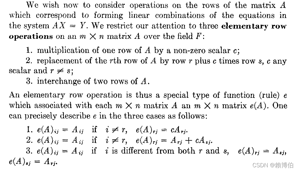 就是中學教科書說的 三個基本的 row 運算 (橫行基本運算) elementrary row operation
- 對某一 row 換成, 該 row 乘上非零之常數
- 對某一 row 換成, 該 row 加上另一row 乘上非零之常數
- 對某兩個 row 置換(互換)
直行基本運算 elementrary column operation, 則是類似的操作, 只是改成對直行操作.
上面所謂轉成一個(等價)的上三角矩陣為何義? 先定義兩個 線性聯立方程組是等價的意思, 定義 兩個 線性聯立方程組是等價的, 如果彼此的方程式互為對方的方程式的線性組合,
則書中有簡單論證, 知道: Theorem1 兩個等價的 線性聯立方程組的解是同樣的, 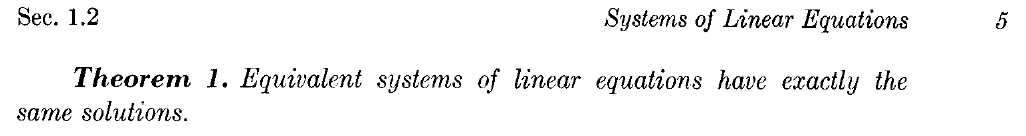 書中接著定義了兩個矩陣是等價的含意, 就是透過有限次三個基本的 row 運算可以將其中一個矩陣轉成另一個矩陣:
 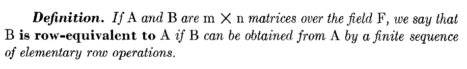 則知道, Gauss Elimination 高斯消去法 是透過基本行列運算 將 線性聯立方程組的 $A$ 矩陣轉成一個的上三角矩陣, 這是與原矩陣等價的, 轉成上三角矩陣後, 線性聯立方程組就很好解了, 得到的解會與原解一致.
Exercises
Ex: 將以下 Maple 的 row operation 的動作用 Python 重寫一次:
AddRow(A, i, j, s)

MultiplyRow(A, i, s)

SwapRow(A, i, j)
Maple 官網 指令的說明: • The AddRow(A, i, j, s) command replaces row i of A with row i + s * row j. This command can also be called as AddRows(A, i, j, s).
• The MultiplyRow(A, i, s) command replaces row i of A with s * row i.
• The SwapRow(A, i, j) command interchanges rows i and j of A. This command can also be called as SwapRows(A, i, j).
Ref: https://www.maplesoft.com/support/help/maple/view.aspx?path=Student%2FLinearAlgebra%2FAddRow link
程式碼實作 : Gauss Elimination 高斯消去法
先觀摩一下 codesansar.com 的程式碼
Ref: https://www.codesansar.com/numerical-methods/gauss-elimination-method-algorithm.htm link
他的程式碼寫的較詳細繁瑣, 容易見樹不見林, 尤其 $A$ 的 entry 輸入是用input 的方法, 在 consola 逐個輸入, 矩陣較大, 就很不方便! (緊接此後面, 本文作者已寫一個簡化版, 方便初學者直接抓住高斯消去法的主要精神及coding.)
以下 codesansar 的程式碼較瑣碎, 可以直接看註解例子說明, 直接抓住感覺
給一線性聯立方程組 \(\begin{array}{c c} 2 \;x_1 &+& 3 \;x_2 &+& 1 \;x_3 &=& 4 \\ 4 \;x_1 &+& 1 \;x_2 &+& -3 \;x_3 &=& -2 \\ -1 \;x_1 &+& 2 \;x_2 &+& 2 \;x_3 &=& 2 \end{array}\) 可以寫下對照之矩陣表法: \(Ax=B\) \(\left( \begin{array}{c c} 2 & 3 & 1 \\ 4 & 1 & -3 \\ -1 & 2 & 2 \\ \end{array} \right) \left( \begin{array}{c c} x_1 \\ x_2 \\ x_3 \\ \end{array} \right) = \left( \begin{array}{c c} 4 \\ -2 \\ 2 \\ \end{array} \right)\\\) where \(A = \left( \begin{array}{c c} 2 & 3 & 1 \\ 4 & 1 & -3 \\ -1 & 2 & 2 \\ \end{array} \right)\\ %A = \begin{pmatrix}10 & -7 & 0 \\ -3 & 2 & 6 \\ 5 & -1 & 5 \\ \end{pmatrix} \\ x = \left( \begin{array}{c c} x_1 \\ x_2 \\ x_3 \\ \end{array} \right)\\ B= \left( \begin{array}{c c} 4 \\ -2 \\ 2 \\ \end{array} \right)\)
##以下先觀摩一下 codesansar,com 的程式碼
##**Ref:** https://www.codesansar.com/numerical-methods/gauss-elimination-method-algorithm.htm [link](https://www.codesansar.com/numerical-methods/gauss-elimination-method-algorithm.htm)
##他的程式碼寫的較詳細繁瑣, 容易見樹不見林,
##緊接此後面, 本文作者已寫一個簡化版, 方便初學者直接抓住高斯消去法的主要精神及coding.
# Ref: CodesSansar
# 河西寫的有分段落, 較清楚, 20210322

# Importing NumPy Library
import numpy as np
import sys

# Reading number of unknowns
n = int(input('Enter number of unknowns: '))

# Making numpy array of n x n+1 size and initializing
# to zero for storing augmented matrix
a = np.zeros((n,n+1))

# Making numpy array of n size and initializing
# to zero for storing solution vector
x = np.zeros(n)

# Reading augmented matrix coefficients
print('Enter Augmented Matrix Coefficients:')
for i in range(n):
    for j in range(n+1):
        a[i][j] = float(input( 'a['+str(i)+']['+ str(j)+']='))

# Applying Gauss Elimination
for i in range(n):
    if a[i][i] == 0.0:
        sys.exit('Divide by zero detected!')

    for j in range(i+1, n):
        ratio = a[j][i]/a[i][i]
        # 此處 codes, 河西寫的有分段落, 較清楚
        for k in range(n+1):
            a[j][k] = a[j][k] - ratio * a[i][k]

# Back Substitution
x[n-1] = a[n-1][n]/a[n-1][n-1]

for i in range(n-2,-1,-1):
    x[i] = a[i][n]

    for j in range(i+1,n):
        x[i] = x[i] - a[i][j]*x[j]

    x[i] = x[i]/a[i][i]

# Displaying solution
print('\nRequired solution is: ')
for i in range(n):
    print('X%d = %0.2f' %(i,x[i]), end = '\t')


##>>>
##= RESTART: C:/Users/user/Desktop/Gauss Elimination Python Program_Codesansar.py
##Enter number of unknowns: 3
##Enter Augmented Matrix Coefficients:
##a[0][0]=2.0
##a[0][1]=3.0
##a[0][2]=1.0
##a[0][3]=4.0
##a[1][0]=4.0
##a[1][1]=1.0
##a[1][2]=-3.0
##a[1][3]=-2.0
##a[2][0]=-1.0
##a[2][1]=2.0
##a[2][2]=2.0
##a[2][3]=2.0
##
##Required solution is:
##X0 = 2.00 X1 = -1.00  X2 = 3.00
由作者改寫的程式碼觀察是否完成上三角矩陣
==以下是作者改寫的程式碼, 會較清楚簡單== 為了更清楚觀察了解程式碼的細節, 我們加寫可以列印出中間上三角矩陣的部分,
# By Prof. P-J Lai MATH NKNU 20220208
#為了更清楚觀察了解程式碼的細節,  我們加寫可以列印出中間上三角矩陣的部分,
#Gauss Elimination_UpperTriangle_Lai.py


# Importing NumPy Library
import numpy as np
import sys

N = 3
A = np.zeros((N,N+1))

A = [[10.0, -7.0, 0, 7.0],
         [-3.0, 2.0, 6.0, 4.0],
         [5.0, -1.0, 5.0, 6.0]]

x = np.zeros(N)

# Applying Gauss Elimination
for i in range(N):
    if A[i][i] == 0.0:
        sys.exit('Divide by zero detected!')

for k in range(0,N):
    pivot = A[k][k] # 取 pivot
    if pivot == 0.0:
        sys.exit('Divide by zero detected!')

    for i in range(k+1, N):
    ##      if i != k:
            d= A[i][k]
            for j1 in range(N+1):
                A[i][j1] = A[i][j1] - d*A[k][j1]/pivot

# 以下觀察是否已清掃成上三角矩陣
for k in range(N):
    for i in range(N+1):
        print("x{}{} = {:.1f}\t".format( k+1,i+1 , A[k][i]), end="\t")
    print("\n")


##輸出:
##>>>
##= RESTART: D:/NEW_筆電的/網路免費軟體資料/Python教學/Python科學計算/線性代數/聯立方程式的解法2_GaussElimination消去法/Gauss Elimination_UpperTriangle_Lai.py
##x11 = 10.0    x12 = -7.0    x13 = 0.0   x14 = 7.0
##
##x21 = 0.0   x22 = -0.1    x23 = 6.0   x24 = 6.1
##
##x31 = 0.0   x32 = 0.0   x33 = 155.0   x34 = 155.0
輸出:
>>>
= RESTART: D:\NEW_筆電的\網路免費軟體資料\Python教學\Python科學計算\線性代數\聯立方程式的解法2_GaussElimination消去法\Gauss Elimination_backwardSubstitution_Lai.py
x11 = 10.0    x12 = -7.0    x13 = 0.0   x14 = 7.0

x21 = 0.0   x22 = -0.1    x23 = 6.0   x24 = 6.1

x31 = 0.0   x32 = 0.0   x33 = 155.0   x34 = 155.0
注意一下以上 print 之呈現: 控制print 印出之小數位數只有一位, 讓視覺較舒服 print("x{}{} = {:.1f}\t".format( k+1,i+1 , A[k][i]), end="\t")
由作者改寫的程式碼接著觀察”後向替代法”之部分
# By Prof. P-J Lai MATH NKNU 20220209

#Gauss Elimination_backwardSubstitution_Lai.py

# Importing NumPy Library
import numpy as np
import sys

N = 3
A = np.zeros((N,N+1))
A = [[10.0, -7.0, 0, 7.0],
         [-3.0, 2.0, 6.0, 4.0],
         [5.0, -1.0, 5.0, 6.0]]

x = np.zeros(N)

# Applying Gauss Elimination
for i in range(N):
    if A[i][i] == 0.0:
        sys.exit('Divide by zero detected!')

for k in range(0,N):
    pivot = A[k][k] # 取 pivot
    if pivot == 0.0:
        sys.exit('Divide by zero detected!')

    for i in range(k+1, N):
    ##      if i != k:
            d= A[i][k]
            for j1 in range(N+1):
                A[i][j1] = A[i][j1] - d*A[k][j1]/pivot

#進行後向替代求出解
# Back Substitution
# 觀摩一下 codesansar,com 的程式碼
# 以下codesansar的程式碼較瑣碎, 可以直接看註解例子說明, 直接抓住感覺
# 可以不拘泥用 augmented matrix,
# 而是把 A 與  b 分開, 對照自己心中高斯消去法的的思緒會較清楚.

x[N-1] = A[N-1][N]/A[N-1][N-1]
# 就是, 例如, x3 = b3/A33

for i in range(N-2,-1,-1):
    x[i] = A[i][N]
    # 就是, 例如, b2

    for j in range(i+1,N):
        x[i] = x[i] - A[i][j]*x[j]
        # A22*x2 = b2 - A23*x3

    x[i] = x[i]/A[i][i]
    # x2 = (b2 - A23*x3)/A22

# Displaying solution
print('\nRequired solution is: ')
for i in range(N):
    #print('X%d = %0.2f' %(i,x[i]), end = '\t')
    print('X{} = {:.2f}'.format(i,x[i]), end = '\t')

##輸出:
##Required solution is:
##X0 = 0.00 X1 = -1.00  X2 = 1.00
輸出:
>>>
= RESTART: D:\NEW_筆電的\網路免費軟體資料\Python教學\Python科學計算\線性代數\聯立方程式的解法2_GaussElimination消去法\Gauss Elimination_backwardSubstitution_Lai.py

Required solution is:
X0 = 0.00 X1 = -1.00  X2 = 1.00
Exercises
Ex: 練習在 consola(終端視窗) 狀態, 一動一動執行, 了解整個過程.
Ex: 如果你已經完成理論那節的習題, 用 Python程式 寫下以下的指令 AddRow(A, i, j, s), MultiplyRow(A, i, s), SwapRow(A, i, j), 試著用此三個指令重寫上面 高斯消去法的程式, 看看是否會==更清楚, 更易閱讀與維護程式碼==.
Ex: 用 list comprehension 重寫, 看看這樣寫出的codes 是否會較清楚直觀.
Ex: 可以不拘泥用 augmented matrix, 而是把 A 與 b 分開, 對照自己心中高斯消去法的的思緒, 看看這樣寫出的codes 是否會較清楚直觀.
程式碼實作 : Gauss-Jordan Elimination 高斯喬丹消去法
- 高斯消去法是用行或列基本運算清掃成上三角矩陣
- Gauss-Jordan 消去法是用行或列基本運算清掃成對角線矩陣
Gauss-Jordan 高斯喬丹消去法 寫成矩陣表法, 就是用行或列基本運算將 A 清掃成對角線矩陣:
\(Ax=B\) \(\left( \begin{array}{c c} a_{11} & a_{12} & a_{13} \\ a_{21} & a_{22} & a_{23} \\ a_{31} & a_{32} & a_{33} \\ \end{array} \right) \left( \begin{array}{c c} x_1 \\ x_2 \\ x_3 \\ \end{array} \right) = \left( \begin{array}{c c} b_{1} \\ b_{2} \\ b_{3} \\ \end{array} \right)\\\) $\stackrel{行列基本運算}{\Longrightarrow}$ \(\left( \begin{array}{c c} 1 & 0 & 0 \\ 0 & 1& 0 \\ 0 & 0 & 1 \\ \end{array} \right) \left( \begin{array}{c c} x_1 \\ x_2 \\ x_3 \\ \end{array} \right) = \left( \begin{array}{c c} b_{1}' \\ b_{2}' \\ b_{3}' \\ \end{array} \right)\\\)
Gauss-Jordan 就是用 $a_{11}$ 去清掃其餘 row, 接著用 $a_{22}$ 去清掃其餘 row (水平的一條叫row, 垂直叫column) (上下方的 row 都清掃), 接著用 $a_{33}$ 去清掃其餘 row, 最後形成一個對角線矩陣, 就可以立即得到解. Gauss elimination 則是只往下方的 row 清掃 (上方的 row 不清掃), 最後形成一個上三角矩陣, 再依序用 “後向代入” 得 $x_3$, $x_2$, $x_1$.
\(\begin{array}{c c} a_{11} \;x_1 &+& a_{12} \;x_2 &+& a_{13} \;x_3 &=& b_{1} \\ a_{21} \;x_1 &+& a_{22} \;x_2 &+& a_{23} \;x_3 &=& b_{2} \\ a_{31} \;x_1 &+& a_{32} \;x_2 &+& a_{33} \;x_3 &=& b_{3}\end{array}\) \(Ax=B\) \(\left( \begin{array}{c c} 2.0 & 3.0 & 1.0 \\ 4.0 & 1.0 & -3.0 \\ -1 & 2 & 2 \\ \end{array} \right) \left( \begin{array}{c c} x_1 \\ x_2 \\ x_3 \\ \end{array} \right) = \left( \begin{array}{c c} 4.0 \\ -2.0 \\ 2.0 \\ \end{array} \right)\\\) where \(A = \left( \begin{array}{c c} 2.0 & 3.0 & 1.0 \\ 4.0 & 1.0 & -3.0 \\ -1 & 2 & 2 \\ \end{array} \right)\\ x = \left( \begin{array}{c c} x_1 \\ x_2 \\ x_3 \\ \end{array} \right)\\ B= \left( \begin{array}{c c} 4.0 \\ -2.0 \\ 2.0 \\ \end{array} \right)\)
Gauss-Jordan 的 codes
Ref:
https://www.codesansar.com/numerical-methods/gauss-jordan-method-python-program-output.htm link 有現成的數值計算的Python codes
河西朝雄: Gauss-Jordan 參考 河西朝雄 Rei15.c, 改寫為 Python codes
以下為作者改寫自河西朝雄的C語言程式碼, 所以風格還是偏向 C 語言的迴圈式風格:
# By Prof. P-J Lai MATH NKNU 20201223
# 聯立方程式的解法1_Gauss-Jordan
# Ref: 河西朝雄 Rei15.c

N = 3
A = [[2.0, 3.0, 1.0, 4.0],
         [4.0, 1.0, -3.0, -2.0],
         [-1.0, 2.0, 2.0, 2.0]]

# 注意, 軸只有 N-1(3個),  每個主軸 row1~row3 分別除一次自己的 pivot, 故loop只做 0~ (N-1)
for k in range(N):
    pivot = A[k][k] # 取 pivot
    # 注意, 將row k 之 第 j 個column 除以 pivot 時, 是對每個 column 都做, 故loop做 0~N
    for j in range(N+1):
        A[k][j] = A[k][j]/pivot # 除以 pivot
    # 注意, 對各個 row 清掃, 只對每個主軸 row 做, row 個數只有 N,  故loop只做 0~ (N-1)
    for i in range(N):
        if i != k:
            d= A[i][k]
             # 注意, 對每個 row 清掃時, 是對每個 column 都做, 故loop做 0~N
            for j1 in range(N+1):
                A[i][j1] = A[i][j1] - d*A[k][j1]


for k in range(N):
    print("x{a} = {b}".format( a=k+1, b=A[k][N]))
print(A)
import numpy as np
A1 = np.array(A)
print(A1)
# 輸出
##>>>
##============== RESTART: C:/Users/user/Desktop/Gauss_Jordan_test.py =============
##x1 = 2.0
##x2 = -1.0
##x3 = 3.0
##[[1.0, 0.0, 0.0, 2.0], [0.0, 1.0, 0.0, -1.0], [-0.0, -0.0, 1.0, 3.0]]
##[[ 1.  0.  0.  2.]
## [ 0.  1.  0. -1.]
## [-0. -0.  1.  3.]]
##<class 'numpy.ndarray'>
Exercises
Ex: 如果你已經完成理論那節的習題: 用 Python程式 寫下以下的指令 AddRow(A, i, j, s), MultiplyRow(A, i, s), SwapRow(A, i, j), 試著用此三個指令重寫上面 高斯消去法的程式, 看看是否會==更清楚, 更易閱讀與維護程式碼==.
改寫為 Python 的 list comprehension 列表解析式的風格
以上是 C 語言的風格 以下改寫為 Python 的 list comprehension 列表解析式的風格
# By Prof. P-J Lai MATH NKNU 20201223
# 聯立方程式的解法1_Gauss-Jordan
# Ref: 河西朝雄 Rei15.c
# 以下用 列表解析式的寫法 list comprehension
# linearEq_1_Gauss-Jordan_listCompreh.py
# [ A[k][j] = A[k][j]/pivot for j in range(N+1)] 不行!

N = 3
A = [[2.0, 3.0, 1.0, 4.0],
         [4.0, 1.0, -3.0, -2.0],
         [-1.0, 2.0, 2.0, 2.0]]

# 注意, 軸只有 N-1個(3個),  每個主軸 row1~row3 分別除一次自己的 pivot, 故loop只做 0~ (N-1)
for k in range(N):
    pivot = A[k][k] # 取 pivot
    # 注意, 將row k 之 第 j 個column 除以 pivot 時, 是對每個 column 都做, 故loop做 0~N
    A[k] = [ A[k][j]/pivot for j in range(N+1)]
    # 注意, 對各個 row 清掃, 只對每個主軸 row 做, row 個數只有 N,  故loop只做 0~ (N-1)
    for i in range(N):
        if i != k:
            d= A[i][k]
             # 注意, 對每個 row 清掃時, 是對每個 column 都做, 故loop做 0~N
            A[i] = [ A[i][j1] - d*A[k][j1] for j1 in range(N+1)]

[ print("x{a} = {b}".format( a=k+1, b=A[k][N])) for k in range(N)]


##>>>
##= RESTART: C:\Users\user\Desktop\linearEq_1_Gauss-Jordan_listCompreh.py
##x1 = 2.0
##x2 = -1.0
##x3 = 3.0
Ex: 以上還可以用列表解析式再進一步簡化,
==但是一般不建議列表解析式的用到含三層或三層以上==, 因為已經不好閱讀了! 同學可以自己試著做看看用到含三層, 看看是否會更好閱讀, 或是閱讀與維護效果不好.
LU 分解
LU 分解可以定義成把高斯消去法的過程寫成演算法, 所以 ==LU 分解根本就是程式化的高斯消去法==.
LU 分解 的現成指令, 只有在 scipy.linalg 與 sympy 有看到,numpy.linalg 則沒有, 兩者都有, cholesky, qr, svd. scipy.linalg 比 numpy.linalg 多了 lu, shur
sympy 中有關 LU 分解的指令
from sympy import *
L, U, _ = A.LUdecomposition()
Ref:
- 陳擎文教學網:python解線性代數, 線性代數第6章 反矩陣inverse, LU分解算聯立方程式, https://acupun.site/lecture/linearAlgebra/pdfBooks/chp6-inverseMatrix.pdf link
- LU 分解 的現成指令, 只有在 scipy.linalg 與 sympy 有看到,numpy.linalg 則沒有, 兩者都有, cholesky, qr, svd. scipy.linalg 多 lu, shur 等 – Numpy linalg 最新列表: https://numpy.org/devdocs/reference/routines.linalg.html link – SciPy linalg 最新列表: https://docs.scipy.org/doc/scipy/reference/linalg.html#scipy.linalg link
- R. L. Burden, J. D. Faires, sec 6.5 p.388, Numerical analysis, Brooks/Cole, 7th ed., 2001
用寫程式的方式實現 LU 分解
以下討論用寫程式的方式實現 LU 分解:
Ref: R. L. Burden, J. D. Faires, sec 6.5 p.388, Numerical analysis, Brooks/Cole, 7th ed., 2001
LU 分解 演算法 的原理
高斯消去法, 可以用來對矩陣進行 LU 分解, 高斯消去法, 消去第一個column 的動作:
\(\begin{array}{c c} a_{11}' \;x_1 &+& a_{12}' \;x_2 &+& a_{13}' \;x_3 &=& b_{1}'\\ \not{a_{21}} \;x_1 &+& a_{22}' \;x_2 &+& a_{23}' \;x_3 &=& b_{2}' \\ \not{a_{31}} \;x_1 &+& a_{32}' \;x_2 &+& a_{33}' \;x_3 &=& b_{3}'\end{array}\) 可以用一個矩陣乘法來表達: \(\begin{pmatrix} 1 & 0 & 0 \\ -m_{21} & 1 & 0 \\ -m_{31} & 0 & 1 & \\ \end{pmatrix} \begin{pmatrix} a_{11} & a_{12} & a_{13} \\ a_{21} & a_{22} & a_{23} \\ a_{31} & a_{32} & a_{33} \\ \end{pmatrix}= \begin{pmatrix} a_{11}' & a_{12}' & a_{13}' \\ 0 & a_{22}' & a_{23}' \\ 0 & a_{32}' & a_{33}' \\ \end{pmatrix}\) Where $m_{j,1}=\frac{a_{j1}}{a_{11}}$
同學可以自己有耐心的在紙上走一遍高斯消去法, 會發現對第一個直行column 往下消的動作: $(E_j - m_{j,1}E_1) \rightarrow E_j, \;j=2,3.$ 確實對照到以下矩陣相乘
\(\begin{pmatrix} 1 & 0 & 0 \\ -m_{21} & 1 & 0 \\ -m_{31} & 0 & 1 & \\ \end{pmatrix} \left( \begin{array}{c c} a_{11} & a_{12} & a_{13} \\ a_{21} & a_{22} & a_{23} \\ a_{31} & a_{32} & a_{33} \\ \end{array} \right)\) 以下我們觀察 對第一個直行column 往下消的過程中, 處理第2個 row 的動作:
$(E_2 - m_{2,1}E_1) \rightarrow E_2$ : \(\begin{array}{c c} a_{11} \;x_1 &+& a_{12} \;x_2 &+& a_{13} \;x_3 &=& b_{1} \\ a_{21} \;x_1 &+& a_{22} \;x_2 &+& a_{23} \;x_3 &=& b_{2} \\ a_{31} \;x_1 &+& a_{32} \;x_2 &+& a_{33} \;x_3 &=& b_{3}\end{array}\)
$m_{2,1}E_1$, 就是先把第一個 row $E_1$ 乘上 $-m_{2,1}=-\frac{a_{21}}{a_{11}}$, 如下 $\Rightarrow$
\[\begin{array}{c c} -\frac{a_{21}}{a_{11}} \times ({a_{11}} \times \;x_1) &+& -\frac{a_{21}}{a_{11}} \times (a_{12} \times \;x_2) &+& -\frac{a_{21}}{a_{11}} \times (a_{13} \times \;x_3) &=& -\frac{a_{21}}{a_{11}} \times (b_{1}) \\ a_{21} \;x_1 &+& a_{22} \;x_2 &+& a_{23} \;x_3 &=& b_{2} \\ a_{31} \;x_1 &+& a_{32} \;x_2 &+& a_{33} \;x_3 &=& b_{3}\end{array}\]$(E_2 - m_{2,1}E_1) \rightarrow E_2$, 再把 第一個 row 加到 第二個 row, 此時我們保持 $E_1$為原來的 $\Rightarrow$
\(\begin{array}{c c} a_{11} \;x_1 &+& a_{12} \;x_2 &+& a_{13} \;x_3 &=& b_{1}\\ (-\frac{a_{21}} {a_{11}} \times {a_{11}} +a_{21}) \;x_1 &+& (-\frac{a_{21}} {a_{11}} \times {a_{12}} + a_{22}) \;x_2 &+& -\frac{a_{21}} {a_{11}} \times a_{13}+a_{23} \;x_3 &=& -\frac{a_{21}} {a_{11}} \times b_{1} +b_{2} \\ a_{31} \;x_1 &+& a_{32} \;x_2 &+& a_{33} \;x_3 &=& b_{3}\end{array}\) 這樣操作之後, 就得到 $a_{2,1}$ 成為 0. \(\begin{pmatrix} a_{11}' & a_{12}' & a_{13}' \\ 0 & a_{22}' & a_{23}' \\ a_{31}' & a_{32}' & a_{33}' \\ \end{pmatrix}\) 類似的, 同學可以手算驗證, 對第一個直行column 往下消的過程中, 處理第 3 個 row 的動作:
$(E_3 - m_{3,1}E_1) \rightarrow E_3$ $m_{3,1}E_1$, 就是先把第一個 row $E_1$ 乘上 $-m_{3,1}=-\frac{a_{31}}{a_{11}}$, 再把 第一個 row 加到 第 3 個 row, $(E_3 - m_{3,1}E_1) \rightarrow E_3$,
就得到 $a_{3,1}$ 成為 0, 如此就完成 第一個直行column 往下消的程序. \(\begin{pmatrix} a_{11}' & a_{12}' & a_{13}' \\ 0 & a_{22}' & a_{23}' \\ 0 & a_{32}' & a_{33}' \\ \end{pmatrix}\)
一般性 n $\times$ n 矩陣的公式, Burden & Faires 書中稱此消去第1個直行column的矩陣為 The first Gaussian transformation matrix 第一個高斯變換矩陣負責清掃第1個直行column: \(M^{(1)}=\begin{pmatrix} 1 & 0 & \cdots & \cdots & 0 \\ -m_{21} & 1 & \ddots & & \vdots \\ \vdots & 0 & \ddots & \ddots & \vdots \\ \vdots & \vdots & \ddots & 1 & 0 \\ -m_{n1} & 0 & \cdots & 0 & 1 & \\ \end{pmatrix},\) Where \(m_{j,1}=\frac{a_{j1}^{(1)}}{a_{11}^{(1)}}\)
消去第k個直行 column 的矩陣 The kth Gaussian transformation matrix 第k個高斯變換矩陣負責清掃第k個直行column: \(M^{(k)}=\begin{pmatrix} 1 &0& 0 & \cdots & \cdots & 0 \\ 0 &1& 0 & \ddots & & \vdots \\ \vdots & 0 & \ddots & \ddots & \ddots & \vdots \\ \vdots & \vdots &-m_{k+1,k} & \ddots & 0 & \vdots \\ \vdots & \vdots & \vdots & \vdots & 1 & 0 & \\ 0 & 0 & -m_{n,k} & 0 & 0 & 1 & \\ \end{pmatrix},\) Where \(m_{j,k}=\frac{a_{jk}^{(k)}}{a_{kk}^{(k)}}\)
透過這一連串的 $M^{(k)}$ 乘上 $A$ 就把 A 轉成上三角. 我們依照 Burden & Faires 書中的符號, 來觀察高斯消去法這一過程: \(Ax=b\) 持續左右兩邊乘上第k個高斯變換矩陣 \(M^{(1)}Ax=M^{(1)}b\) \(M^{(k)}\cdots M^{(1)} Ax=M^{(k)}\cdots M^{(1)}b\) \(M^{(n-1)}\cdots M^{(k)}\cdots M^{(1)} Ax=M^{(n-1)}\cdots M^{(k)}\cdots M^{(1)}b\) 則知 上式左邊已經是轉成上三角了, 令為 $U$. \(U=M^{(n-1)}\cdots M^{(1)} A\) 而 $U$ 可以透過真實的乘上 $M^{(n-1)}\cdots M^{(1)} A$ 去得到: \(M^{(n-1)}\cdots M^{(1)} A=U\) 實際小矩陣的解題, 也可以透過我們熟悉的高斯消去法對$A$得到的上三角矩陣, 透過這種方式去得到 $U$. 我們再進一步觀察, 左右兩邊同時乘上 $(M^{(k)})^{-1}$, 讓 $A$ 的分解長相呈現出來: \((M^{(n-1)})^{-1}M^{(n-1)}M^{(n-2)}\cdots M^{(1)} A=(M^{(n-1)})^{-1}U\) \(M^{(n-2)}\cdots M^{(1)} A=(M^{(n-1)})^{-1}U\) \((M^{(n-2)})^{-1}M^{(n-2)}\cdots M^{(1)} A=(M^{(n-2)})^{-1}(M^{(n-1)})^{-1}U\) 最終得到 $A$ 的分解長相 \(A=(M^{(1)})^{-1} \cdots (M^{(n-2)})^{-1}(M^{(n-1)})^{-1}U\) 如果 \((M^{(1)})^{-1} \cdots (M^{(n-2)})^{-1}(M^{(n-1)})^{-1}\) 是一個下三角矩陣, 符號命名為 $L$, 則我們就完成
\(A = L \times U\) 的 LU 分解了!
$(M^{(1)})^{-1} \cdots (M^{(n-2)})^{-1}(M^{(n-1)})^{-1}$ 是一個下三角矩陣答案是明顯的, 因為上三角矩陣的反矩陣就是下三角矩陣(自己照反矩陣的公式走一下), 所以 \(L=(M^{(1)})^{-1} \cdots (M^{(n-2)})^{-1}(M^{(n-1)})^{-1}\) 確實是一個下三角矩陣, 所以 $A = L \times U$ 的 LU 分解確實完成了!
而 $L$ 必須透過真實的乘上 $(M^{(1)})^{-1} \cdots (M^{(n-2)})^{-1}(M^{(n-1)})^{-1}$ 去得到: \(L=(M^{(1)})^{-1} \cdots (M^{(n-2)})^{-1}(M^{(n-1)})^{-1}\) 可以寫下明確的公式. 由以上的觀查, $LU$ 就可以直接寫下公式去求得, 此部分就是演算法的核心.
LU 分解 演算法
Algorithm 6.4 Direct Factorization To factor the n$\times$n matrix $A=(a_{ij})$ into the product of the lower-triangular matrix $L=(l_{ij})$ and the upper-triangular matrix $U=(u_{ij})$, that is, $A=LU$, where the main diagonal of either $L$ or $U$ is given: INPUT dimension n; the entries $a_{ij}$, $1\le i, j \le n$, of $A$; the diagonal $l_{11},\dots,l_{nn}$ of $L$ or the diagonal $u_{11},\dots,u_{nn}$ of $U$. OUTPUT the entries $l_{ij}$, $1\le j \le i, 1\le i \le n$ of $L$ and the entries $u_{ij}$, $1\le j \le n, 1\le i \le n$ of $U$.
- STEP1
- STEP2
- STEP3 * STEP4 * STEP5
- STEP6
- STEP7
以下是 R. L. Burden, J. D. Faires 書附的 LU 分解的 Matlab codes:
% DIRECT FACTORIZATION ALGORITHM 6.4
%
% To factor the n by n matrix A = (A(I,J)) into the product of the
% lower triangular matrix L = (L(I,J)) and the upper triangular
% matrix U = (U(I,J)), that is A = LU, where the main diagonal of
% either L or U consists of all ones:
%
% INPUT:   dimension n; the entries A(I,J), 1<=I, J<=n, of A;
%          the diagonal L(1,1), ..., L(N,N) of L or the diagonal
%          U(1,1), ..., U(N,N) of U.
%
% OUTPUT:  the entries L(I,J), 1<=J<=I, 1<=I<=n of L and the entries
%          U(I,J), I<=J<=n, 1<=I<=n of U.
 syms('AA', 'NAME', 'INP', 'OK', 'N', 'I', 'J', 'A');
 syms('FLAG', 'ISW', 'XL', 'M', 'KK', 'S', 'K', 'JJ');
 syms('SS', 'OUP', 's');
 TRUE = 1;
 FALSE = 0;
 fprintf(1,'This is the general LU factorization method.\n');
 fprintf(1,'The array will be input from a text file in the order:\n');
 fprintf(1,'A(1,1), A(1,2), ..., A(1,N), \n')
 fprintf(1,'A(2,1), A(2,2), ..., A(2,N),\n');
 fprintf(1,'..., A(N,1), A(N,2), ..., A(N,N)\n\n');
 fprintf(1,'Place as many entries as desired on each line, but separate\n');
 fprintf(1,'entries with\n');
 fprintf(1,'at least one blank.\n\n\n');
 fprintf(1,'Has the input file been created? - enter Y or N.\n');
 AA = input(' ','s');
 if AA == 'Y' | AA == 'y'
 fprintf(1,'Input the file name in the form - drive:\\name.ext\n');
 fprintf(1,'for example:   A:\\DATA.DTA\n');
 NAME = input(' ','s');
 INP = fopen(NAME,'rt');
 OK = FALSE;
 while OK == FALSE
 fprintf(1,'Input the dimension n - an integer.\n');
 N = input(' ');
 if N > 0
 A = zeros(N,N);
 XL = zeros(1,N);
 for I = 1 : N
 for J = 1 : N
 A(I,J) = fscanf(INP, '%f',1);
 end;
 end;
 OK = TRUE;
 fclose(INP);
 else fprintf(1,'The number must be a positive integer.\n');
 end;
 end;
 fprintf(1,'Choice of diagonals:\n');
 fprintf(1,'1. Diagonal of L consists of ones\n');
 fprintf(1,'2. Diagonal of U consists of ones\n');
 fprintf(1,'Please enter 1 or 2.\n');
 FLAG = input(' ');
 if FLAG == 1
 ISW = 0;
 else
 ISW = 1;
 end
 else
 fprintf(1,'The program will end so the input file can be created.\n');
 OK = FALSE;
 end;
 if OK == TRUE
 for I = 1 : N
 XL(I) = 1;
 end;
% STEP 1
 if abs(A(1,1)) <= 1.0e-20
 OK = FALSE;
 else
% the entries of L below the main diagonal will be placed
% in the corresponding entries of A; the entries of U
% above the main diagonal will be placed in the
% corresponding entries of A; the main diagonal which
% was not input will become the main diagonal of A;
% the input main diagonal of L or U is,
% of course, placed in XL
 A(1,1) = A(1,1)/XL(1);
% STEP 2
 for J = 2 : N
 if ISW == 0
% first row of U
 A(1,J) = A(1,J)/XL(1);
% first column of L
 A(J,1) = A(J,1)/A(1,1);
 else
% first row of U
 A(1,J) = A(1,J)/A(1,1);
% first column of L
 A(J,1) = A(J,1)/XL(1);
 end;
 end;
% STEP 3
 M = N-1;
 I = 2;
 while I <= M & OK == TRUE
% STEP 4
 KK = I-1;
 S = 0;
 for K = 1 : KK
 S = S-A(I,K)*A(K,I);
 end;
 A(I,I) = (A(I,I)+S)/XL(I);
 if abs(A(I,I)) <= 1.0e-20
 OK = FALSE;
 else
% STEP 5
 JJ = I+1;
 for J = JJ : N
 SS = 0;
 S = 0;
 for K = 1 : KK
 SS = SS-A(I,K)*A(K,J);
 S = S-A(J,K)*A(K,I);
 end;
 if ISW == 0
% Ith row of U
 A(I,J) = (A(I,J)+SS)/XL(I);
% Ith column of L
 A(J,I) = (A(J,I)+S)/A(I,I);
 else
% Ith row of U
 A(I,J) = (A(I,J)+SS)/A(I,I);
% Ith column of L
 A(J,I) = (A(J,I)+S)/XL(I);
 end;
 end;
 end;
 I = I+1;
 end;
 if OK == TRUE
% STEP 6
 S = 0;
 for K = 1 : M
 S = S-A(N,K)*A(K,N);
 end;
 A(N,N) = (A(N,N)+S)/XL(N);
% If A(N,N) = 0 then A = LU but the matrix is singular.
% Process is complete, all entries of A have been determined.
% STEP 7
 fprintf(1,'Choice of output method:\n');
 fprintf(1,'1. Output to screen\n');
 fprintf(1,'2. Output to text file\n');
 fprintf(1,'Please enter 1 or 2\n');
 FLAG = input(' ');
 if FLAG == 2
 fprintf(1,'Input the file name in the form - drive:\\name.ext\n');
 fprintf(1,'For example   A:\\OUTPUT.DTA\n');
 NAME = input(' ','s');
 OUP = fopen(NAME,'wt');
 else
 OUP = 1;
 end;
 fprintf(OUP, 'GENERAL LU FACTORIZATION\n\n');
 if ISW == 0
 fprintf(OUP, 'The diagonal of L consists of all entries = 1.0\n');
 else
 fprintf(OUP, 'The diagonal of U consists of all entries = 1.0\n');
 end;
 fprintf(OUP, '\nEntries of L below/on diagonal and entries of U above');
 fprintf(OUP, '/on diagonal\n');
 fprintf(OUP, '- output by rows in overwrite format:\n');
 for I = 1 : N
 for J = 1 : N
 fprintf(OUP, ' %11.8f', A(I,J));
 end;
 fprintf(OUP, '\n');
 end;
 if OUP ~= 1
 fclose(OUP);
 fprintf(1,'Output file %s created successfully \n',NAME);
 end;
 end;
 end;
 if OK == FALSE
 fprintf(1,'The matrix does not have an LU factorization.\n');
 end;
 end;
LU 分解定理
==甚麼條件下, 一個矩陣一定保證, 存在 LU 分解?==
Ref: R. L. Burden, J. D. Faires, sec 6.5 p.365, Numerical analysis, Brooks/Cole, 7th ed., 2001.
Theorem 6.17 LU 分解定理 假設 $Ax=b$ 可 以執行高斯消去法, 且在執行高斯消去法時, 無須做 row 的置換(無須挑選 非零的pivot 元素), 則 A 可以分解為 上三角矩陣與下三角矩陣相乘,
\(A=L \times U\) \(U==\begin{pmatrix} a_{11}^{(1)} & a_{12}^{(1)}& a_{13}^{(1)} & \cdots & \cdots & a_{1n}^{(1)} \\ 0 & a_{22}^{(2)} & \ddots & \ddots & & \vdots \\ \vdots & \ddots & \ddots & \ddots & \ddots & \vdots \\ \vdots & \vdots &0 & \ddots & \ddots & \vdots \\ \vdots & \vdots & \vdots & \vdots & a_{n-1,n-1}^{(n-1)} & a_{n-1,n}^{(n-1)} & \\ 0 & \cdots & 0 & \cdots & 0 & a_{n,n}^{(n)} & \\ \end{pmatrix},\), \(L=\begin{pmatrix} 1 &0& 0 & \cdots & \cdots & 0 \\ m_{21} &1& 0 & \ddots & & \vdots \\ \vdots & \ddots & \ddots & \ddots & \ddots & \vdots \\ \vdots & \vdots &m_{k+1,k} & \ddots & 0 & \vdots \\ \vdots & \vdots & \vdots & \vdots & 1 & 0 & \\ m_{n1} & \cdots & m_{n,k} & \cdots & m_{n,n-1} & 1 & \\ \end{pmatrix},\) Where \(m_{j,k}=\frac{a_{jk}^{(k)}}{a_{kk}^{(k)}}\), and $a_{j,k}^{(i)}$ is the ith iteration $a_{i,k}$
以上 Burden and Faires 給的條件是 ==假設 $Ax=b$ 可以執行高斯消去法==, 等,
在 Ref: Kincaid and Cheney, sec 4.2, P.156,Theorem1, Numerical analysis, Brooks/Cole, 3th ed., 2002, 所提的定理Theorem1, 它的前提條件是: ==all n leading principal minors of the n$\times$n matrix A are nonsingular== Theorem1 Theorem on LU-Decomposition If all n leading principal minors of the n$\times$n matrix A are nonsingular, then $A$ has an LU-decomposition.
Appendix
\begin{bmatrix}
以前我學 Latex 寫矩陣, 標準的寫法有點麻煩, 使用 \begin{array}
A = \left( \begin{array}{c c} 10 & -7 & 0 \\ -3 & 2 & 6 \\ 5 & -1 & 5 \\ \end{array} \right)\\
\(A = \left( \begin{array}{c c} 10 & -7 & 0 \\ -3 & 2 & 6 \\ 5 & -1 & 5 \\ \end{array} \right)\)
現在可以用 \begin{pmatrix} 左右小括號矩陣
$$ A =
\begin{pmatrix}
10 & -7 & 0 \\
-3 & 2 & 6 \\
5 & -1 & 5 \\
\end{pmatrix} $$
\(A = \begin{pmatrix}10 & -7 & 0 \\ -3 & 2 & 6 \\ 5 & -1 & 5 \\ \end{pmatrix}\) \begin{bmatrix} 左右中括號矩陣
$$
A =
\begin{bmatrix}
10 & -7 & 0 \\
-3 & 2 & 6 \\
5 & -1 & 5 \\
\end{bmatrix}
$$
\begin{Bmatrix} 左右 大括號矩陣
$$A = \begin{Bmatrix}10 & -7 & 0 \\ -3 & 2 & 6 \\ 5 & -1 & 5 \\ \end{Bmatrix} $$
\(A = \begin{Bmatrix}10 & -7 & 0 \\ -3 & 2 & 6 \\ 5 & -1 & 5 \\ \end{Bmatrix}\)
\begin{vmatrix} 左右絕對值括號矩陣
$$A = \begin{vmatrix}10 & -7 & 0 \\ -3 & 2 & 6 \\ 5 & -1 & 5 \\ \end{vmatrix} $$
\(A = \begin{vmatrix}10 & -7 & 0 \\ -3 & 2 & 6 \\ 5 & -1 & 5 \\ \end{vmatrix}\)
\begin{Vmatrix} 左右雙絕對值(norm)括號矩陣
$$A = \begin{Vmatrix}10 & -7 & 0 \\ -3 & 2 & 6 \\ 5 & -1 & 5 \\ \end{Vmatrix} $$
\(A = \begin{Vmatrix}10 & -7 & 0 \\ -3 & 2 & 6 \\ 5 & -1 & 5 \\ \end{Vmatrix}\)
控制print 印出之小數位數只有一位
注意一下以上print 之呈現: 控制print 印出之小數位數只有一位, 讓視覺較舒服 print("x{}{} = {:.1f}\t".format( k+1,i+1 , A[k][i]), end="\t")
scipy.linalg 中有關矩陣分解的指令
Decompositions :
lu(a[, permute_l, overwrite_a, check_finite])
Compute pivoted LU decomposition of a matrix.
lu_factor(a[, overwrite_a, check_finite])
Compute pivoted LU decomposition of a matrix.
lu_solve(lu_and_piv, b[, trans, …])
Solve an equation system, a x = b, given the LU factorization of a
svd(a[, full_matrices, compute_uv, …])
Singular Value Decomposition.
svdvals(a[, overwrite_a, check_finite])
Compute singular values of a matrix.
diagsvd(s, M, N)
Construct the sigma matrix in SVD from singular values and size M, N.
orth(A[, rcond])
Construct an orthonormal basis for the range of A using SVD
null_space(A[, rcond])
Construct an orthonormal basis for the null space of A using SVD
ldl(A[, lower, hermitian, overwrite_a, …])
Computes the LDLt or Bunch-Kaufman factorization of a symmetric/ hermitian matrix.
cholesky(a[, lower, overwrite_a, check_finite])
Compute the Cholesky decomposition of a matrix.
cholesky_banded(ab[, overwrite_ab, lower, …])
Cholesky decompose a banded Hermitian positive-definite matrix
cho_factor(a[, lower, overwrite_a, check_finite])
Compute the Cholesky decomposition of a matrix, to use in cho_solve
cho_solve(c_and_lower, b[, overwrite_b, …])
Solve the linear equations A x = b, given the Cholesky factorization of A.
cho_solve_banded(cb_and_lower, b[, …])
Solve the linear equations A x = b, given the Cholesky factorization of the banded Hermitian A.
polar(a[, side])
Compute the polar decomposition.
qr(a[, overwrite_a, lwork, mode, pivoting, …])
Compute QR decomposition of a matrix.
qr_multiply(a, c[, mode, pivoting, …])
Calculate the QR decomposition and multiply Q with a matrix.
qr_update(Q, R, u, v[, overwrite_qruv, …])
Rank-k QR update
qr_delete(Q, R, k, int p=1[, which, …])
QR downdate on row or column deletions
qr_insert(Q, R, u, k[, which, rcond, …])
QR update on row or column insertions
rq(a[, overwrite_a, lwork, mode, check_finite])
Compute RQ decomposition of a matrix.
qz(A, B[, output, lwork, sort, overwrite_a, …])
QZ decomposition for generalized eigenvalues of a pair of matrices.
ordqz(A, B[, sort, output, overwrite_a, …])
QZ decomposition for a pair of matrices with reordering.
schur(a[, output, lwork, overwrite_a, sort, …])
Compute Schur decomposition of a matrix.
rsf2csf(T, Z[, check_finite])
Convert real Schur form to complex Schur form.
hessenberg(a[, calc_q, overwrite_a, …])
Compute Hessenberg form of a matrix.
cdf2rdf(w, v)
Converts complex eigenvalues w and eigenvectors v to real eigenvalues in a block diagonal form wr and the associated real eigenvectors vr, such that.
cossin(X[, p, q, separate, swap_sign, …])
Compute the cosine-sine (CS) decomposition of an orthogonal/unitary matrix.
See also
scipy.linalg.interpolative – Interpolative matrix decompositions
References
- R. L. Burden, J. D. Faires, Numerical analysis, Brooks/Cole, 7th ed., 2001.
Kincaid and Cheney, sec 4.2, P.156,Theorem1, Numerical analysis, Brooks/Cole, 3th ed., 2002.
Clever B Moler, Numerical computing with Matlab Moler的書: Ch2 線性代數
Python Numpy全世界最長基礎教程最適合小白學習 還詳細很全速拿, https://twgreatdaily.com/AhWyTG8BMH2_cNUgWU4g.html link.
推薦: 這裡有很具體的指令用法, 用在線性代數課程上: 陳擎文教學網:python解線性代數, https://acupun.site/lecture/linearAlgebra/index.htm link
https://www.codesansar.com/numerical-methods/gauss-jordan-method-python-program-output.htm link 有現成的數值計算的Python codes
- 河西朝雄
https://www.maplesoft.com/support/help/maple/view.aspx?path=Student%2FLinearAlgebra%2FAddRow link
LU 分解 的現成指令, 只有在 scipy 與 sympy 有看到, NumPy 則沒有, 陳擎文教學網:python解線性代數, 線性代數第6章 反矩陣inverse, LU分解算聯立方程式, https://acupun.site/lecture/linearAlgebra/pdfBooks/chp6-inverseMatrix.pdf link
- LU 分解 的現成指令, 只有在 scipy.linalg 與 sympy 有看到, numpy.linalg 則沒有, 兩者都有, cholesky, qr, svd. scipy.linalg 多 lu, shur – Numpy linalg 最新列表: https://numpy.org/devdocs/reference/routines.linalg.html link – SciPy linalg 最新列表: https://docs.scipy.org/doc/scipy/reference/linalg.html#scipy.linalg link – SciPy linalg Decompositions(矩陣分解) 最新列表:
https://docs.scipy.org/doc/scipy/reference/linalg.html#decompositions link
用 Python+Numpy+scipy 執行矩陣計算 9 解線性方程組 迭代法: Jacobi iterated,Gauss-Seidel 等
求解線性聯立方程組之迭代法
迭代法起源於19世紀末, 在小尺度的求解線性聯立方程組, 較少用, 因為時間遠比直接法要久, 但是對於大型線性聯立方程組且要求高精度且帶有 0 的entry, 迭代法運用計算機的效能要遠高於直接法, 迭帶法意指透過同樣的演算程序一直迭帶, 得到越來越精確的解, 類似固定點定理的想法, 求解的步驟, 形如 一個迭代函數:
\(x^{(k)}=T x^{(k-1)} + c , \text{where } x^0 \text{ is some initial vector}.\) 通過輸入一個任意或適當之起始向量 $x^0$, 不斷進行迭代, 得到越來越精確的近似解. 直接法就不是逐步逼近, 而是透過一定計算步驟之後就得到精確解, 例如 中學熟知的 Gauss Elimination(高斯消去法), Gauss-Jordan 等等.
Ref: R. L. Burden, J. D. Faires, Numerical analysis, Brooks/Cole, 7th ed., 2001.
Jacobi iterated method
==以下用 GeoGebra 繪製 Jacobi iterated 流程的說明圖==, 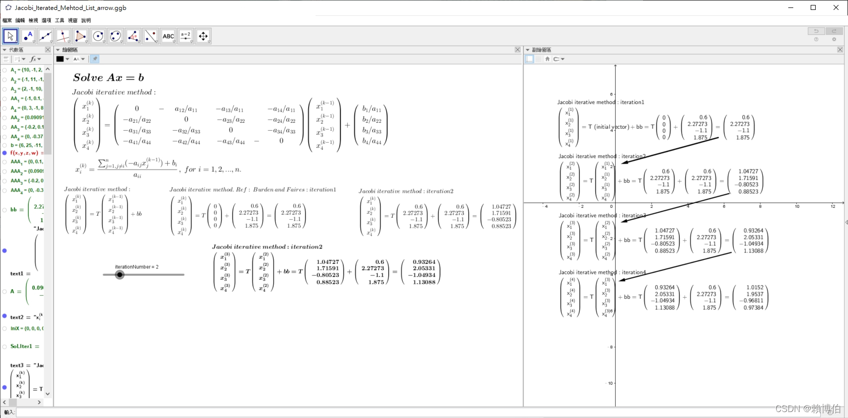
注意, 下圖第 2 步驟的符號有打錯, 待作者修正 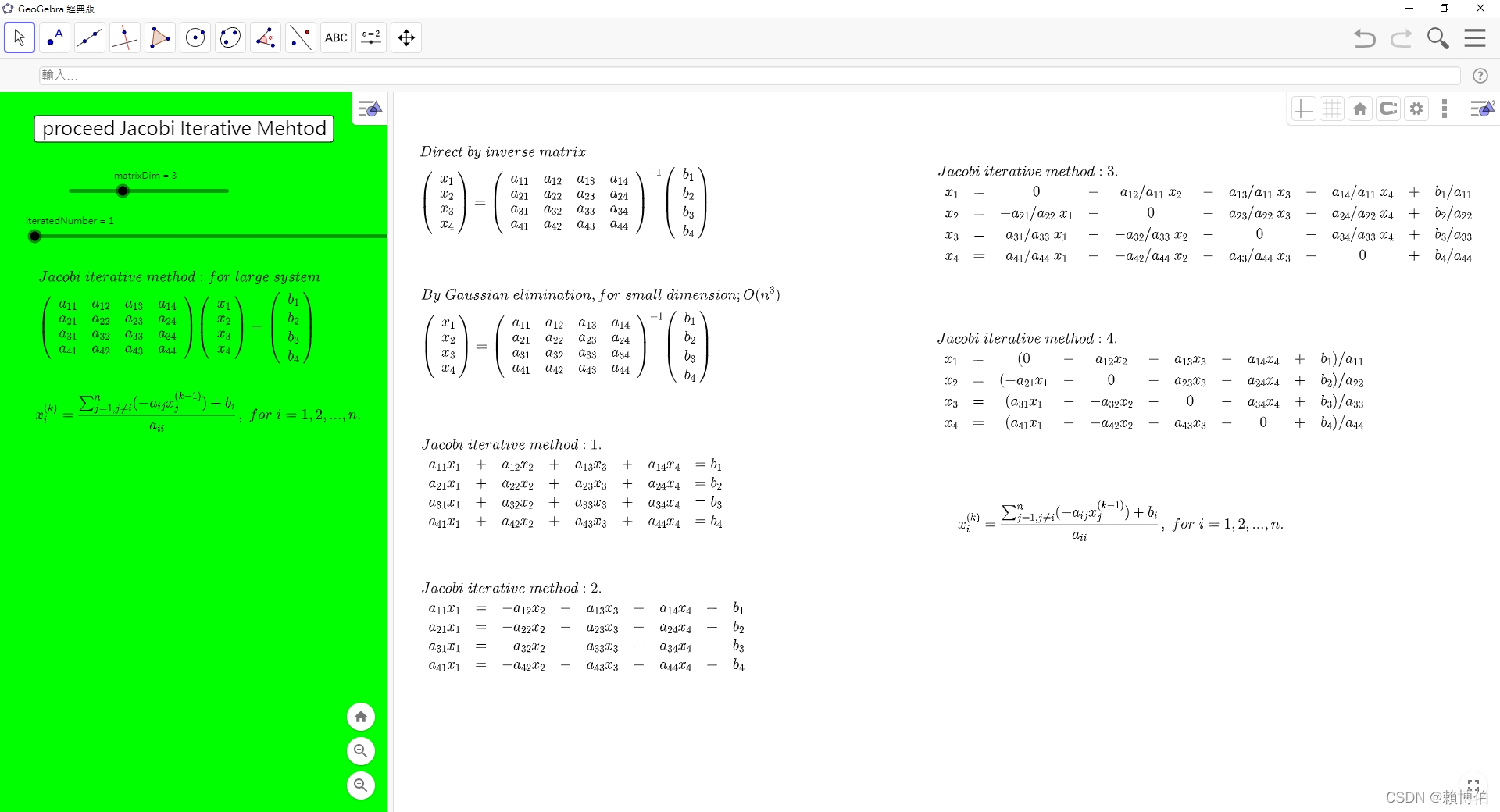
我們先參考 codesansar 站的 程式碼
Ref: https://www.codesansar.com/numerical-methods/python-program-jacobi-iteration-method.htm link
# JacobiMethod_Codesansar.py
# Python Source Code: Jacobi Method
# Defining equations to be solved
# in diagonally dominant form
# Ex: 將以下的 codes 改成 input 一個  numpy array(n by n) 20220130

# 20x + y - 2z = 17
# 3x + 20y -z = -18
# 2x - 3y + 20z = 25

f1 = lambda x,y,z: (17-y+2*z)/20
f2 = lambda x,y,z: (-18-3*x+z)/20
f3 = lambda x,y,z: (25-2*x+3*y)/20

# Initial setup
x0 = 0
y0 = 0
z0 = 0
count = 1
e1 = 100
e2 = 100
e3 = 100

# Reading tolerable error
e = float(input('Enter tolerable error: '))

# Implementation of Jacobi Iteration
print('\nCount\tx\ty\tz\n')

#condition = True
condition = e1>e and e2>e and e3>e

while condition:
    x1 = f1(x0,y0,z0)
    y1 = f2(x0,y0,z0)
    z1 = f3(x0,y0,z0)
    print('%d\t%0.4f\t%0.4f\t%0.4f\n' %(count, x1,y1,z1))
    e1 = abs(x0-x1);
    e2 = abs(y0-y1);
    e3 = abs(z0-z1);

    x0 = x1
    y0 = y1
    z0 = z1

    condition = e1>e and e2>e and e3>e

    count += 1

# 20210321 test
##>>>
##= RESTART: C:\data\NEW\網路免費軟體資料\Python教學\Python科學計算\線性代數\聯立方程式的解法3_JacobiIterated\JacobiMethod_Codesansar.py
##Enter tolerable error: 0.000001
##
##Count x y z
##
##1 0.8500  -0.9000 1.2500
##
##2 1.0200  -0.9650 1.0300
##
##3 1.0012  -1.0015 1.0032
##
##4 1.0004  -1.0000 0.9996
##
##5 1.0000  -1.0001 1.0000
##
##6 1.0000  -1.0000 1.0000
##
##7 1.0000  -1.0000 1.0000
Ex: 將以上的 codes 改成 input 一個 numpy array(n by n).
Gauss-Seidel iterated method
我們先參考 codesansar 站的 程式碼
Ref: https://www.codesansar.com/numerical-methods/python-program-gauss-seidel-iteration-method.htm link
# Ref: https://www.codesansar.com/numerical-methods/python-program-gauss-seidel-iteration-method.htm
# GaussSeidel_Codesansar.py
# Python Source Code: Gauss Seidel Method

# Gauss Seidel Iteration

# Defining equations to be solved
# in diagonally dominant form
f1 = lambda x,y,z: (17-y+2*z)/20
f2 = lambda x,y,z: (-18-3*x+z)/20
f3 = lambda x,y,z: (25-2*x+3*y)/20

# Initial setup
x0 = 0
y0 = 0
z0 = 0
count = 1

# Reading tolerable error
e = float(input('Enter tolerable error: '))

# Implementation of Gauss Seidel Iteration
print('\nCount\tx\ty\tz\n')

condition = True

while condition:
    x1 = f1(x0,y0,z0)
    # 與 Jacobi 不同之處在 Jacobi是 y1 = f2(x0,y0,z0)
    # Gauss Seidel 是 y1 = f2(x1,y0,z0), i.e., 立即使用新的 x1
    # 20201225
    y1 = f2(x1,y0,z0)
    z1 = f3(x1,y1,z0)
    print('%d\t%0.4f\t%0.4f\t%0.4f\n' %(count, x1,y1,z1))
    e1 = abs(x0-x1);
    e2 = abs(y0-y1);
    e3 = abs(z0-z1);

    count += 1
    x0 = x1
    y0 = y1
    z0 = z1

    condition = e1>e and e2>e and e3>e

print('\nSolution: x=%0.3f, y=%0.3f and z = %0.3f\n'% (x1,y1,z1))


##>>>
##= RESTART: C:\Users\user\Desktop\202102上課\聯立方程式的解法4_GaussSeidel\GuassSeidel_Codesansar.py
##Enter tolerable error: 0.00001
##
##Count x y z
##
##1 0.8500  -1.0275 1.0109
##
##2 1.0025  -0.9998 0.9998
##
##3 1.0000  -1.0000 1.0000
##
##4 1.0000  -1.0000 1.0000
##
##
##Solution: x=1.000, y=-1.000 and z = 1.000
References
R. L. Burden, J. D. Faires, Numerical analysis, Brooks/Cole, 7th ed., 2001.
https://www.codesansar.com/numerical-methods/python-program-jacobi-iteration-method.htm link
Clever B Moler, Numerical computing with Matlab Moler的書: Ch2 線性代數
Python Numpy全世界最長基礎教程最適合小白學習 還詳細很全速拿, https://twgreatdaily.com/AhWyTG8BMH2_cNUgWU4g.html link.
推薦: 這裡有很具體的指令用法, 用在線性代數課程上: 陳擎文教學網:python解線性代數, https://acupun.site/lecture/linearAlgebra/index.htm link
https://www.codesansar.com/numerical-methods/gauss-jordan-method-python-program-output.htm link 有現成的數值計算的Python codes
河西朝雄
20250306 revised
用 Python+SciPy+SymPy+GeoGebra 執行微積分計算
- GeoGebra 在中學數理科到大二微積分相當夠用
- Python 中執行矩陣運算的主力是 NumPy
- Python 中執行數值計算的主力是 SciPy(先載入NumPy)
- Python 中執行微積分或符號運算的主力是 SymPy, 註: 符號計算 相當於叫電腦模擬我們中學或大學時用手算出數學公式的計算
如果考量到
- 免費開源社群穩定
- 兼具數值與符號運算
- 又能延伸到研究所
建議使用 GeoGebra 同時搭配 Python+(先載入)NumPy(矩陣)+SciPy(科學計算)+SymPy(符號運算), (如果是GeoGebra 搭配 以下之軟體,可能數值與符號運算就無法兼具,
- GeoGebra 搭配 以下之免費軟體, : GeoGebra + R (偏重統計與數值), GeoGebra + Octave (偏重數值), GeoGebra + Maxima (偏重符號運算) 等,
- 如果不在意付費, 則搭配付費軟體, 學習曲線會較低, 因為付費軟體通常說明文檔會較齊全貼心: GeoGebra + Matlab (偏重數值), GeoGebra + Maple (偏重符號運算), GeoGebra + Mathematica (偏重符號運算) 搭配, 都可.)
建議初學者使用何種軟體教微積分或計算微積分
最好是同時使用 GeoGebra 與一個程式語言類型的軟體
例如 GeoGebra 搭配 Python(+Scipy(NumPy)+SymPy) 依照本人教授微積分多年, 嘗試用各種軟體製作教材同時並教會同學使用, 以輔助同學自我學習, 我目前得到的心得是: 最好是同時使用 GeoGebra 與一個程式語言類型的軟體, 例如 GeoGebra 搭配 Python(+Scipy(先載入NumPy)+SymPy), 或 GeoGebra 搭配 Matlab, Maple, Mathematica 或 Octave, R, Maxima 等搭配, 都可, Matlab, Maple, Mathematica 是付費的, 另外近年, 還有Julia 網路常介紹.
我自己的建議是可以兩方搭配一起用, 當然學習的時間, 以我本人的經驗, 教師以課餘瑣碎的時間邊教邊摸索自學, 約需1~3年的時間(單只有GeoGebra, 在有熟悉的人帶領學習或在旁邊可以隨時發問的前提下只需2,3 個月, 如果完全自己摸索沒人可以問, 可能要半年才能製作較進階的GeoGebra 內容, 至於 Python+NumPy+SciPy+SymPy 等, Python 雖然好學, 但是要掌握這麼多的工具箱, 還是要不短的時間, 如果完全自己摸索沒人可以問, 假設連 Python 也是從頭學, 可能至少要半年, 才能製作基礎的教材, 閒暇有空就學, 應該 1 年多就可以進入熟悉的狀態, 加上前面的 GeoGebra 半年的時間, 合計約至少兩年差不多, 另外 Python+NumPy+SciPy+SymPy 如果有人教或有跟隨課程應該半年就可以基本夠用了), 但是, 作者觀察本校師範院校教出的學生, 尤其是我自己教過的同學進入各中小學教書, 如果不肯把握時間加緊自學(中小學教學上處理學生的瑣事很多, 時不時有一堆表面功夫的研習必須參加, 應校長要求申請計畫, 應付上級督導等, 必須是對使用軟體輔助數學探索有熱愛且學習意志力很堅定的老師), 過了10年, 發現這個學生還是不會駕馭軟體協助自己教學與研究, 只能羨慕自己的同事, 輕易嫻熟的操控軟體做出精美的數學教材, 電腦這樣的東西, 花時間敲指令下去就有收穫, 所謂 “拳打千遍, 身法自然 “, 如果用看的用想的, 永遠只能羨慕別人.
GeoGebra 在中學數理科到大一微積分相當夠用
GeoGebra 可以直接以滑鼠拖拉畫圖, 以滑桿功能展示即時動態變化(動畫), 也有不少微積分的指令, 例如以下我用 GeoGebra 製作的積分的動態展示, 加上文字說明, 按鈕等, 同樣的效果, 如果僅是靜態圖, 用 Python+Matplotlib 的 pyplot畫, 恐怕要花上兩三倍的時間. 而且下圖之 Geogebra 的圖是可以拖動滑桿, 改變切割區間之粗細, 動態演示的, 這種動畫效果, 如果要用 Python+Matplotlib 的 pyplot 畫呈現, 會花上更多倍時間, 且需要對 Matplotlib 有更多的了解與熟悉. (更正: 下圖中的說明 “長方形法” 其實是”梯形法”) 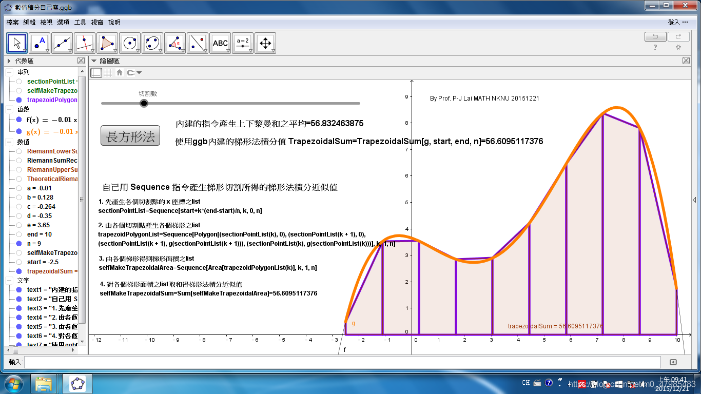 例如以下是我用 GeoGebra 製作的 微積分考卷的圖, 要呈現 Varberg 微積分那本原文教科書的某題之圖, 加上自己的設計, 用 GeoGebra 製作 3D 函數圖也很輕鬆:
 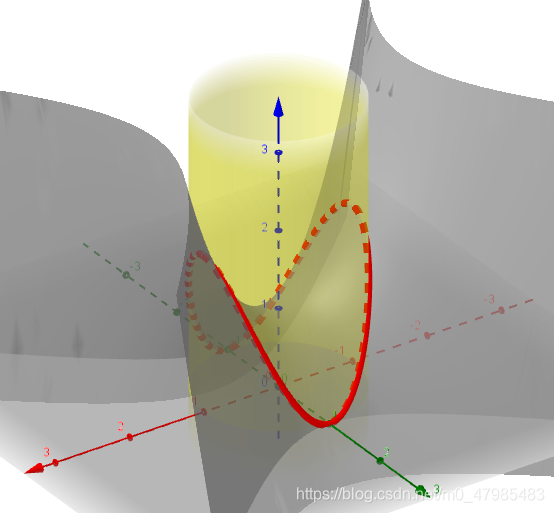 或, 以下是用 GeoGebra 製作的 兩變數函數 $f(x,y)=4+xy-x^2-y^2$ 侷限在單位圓上求極值, 的說明圖:
 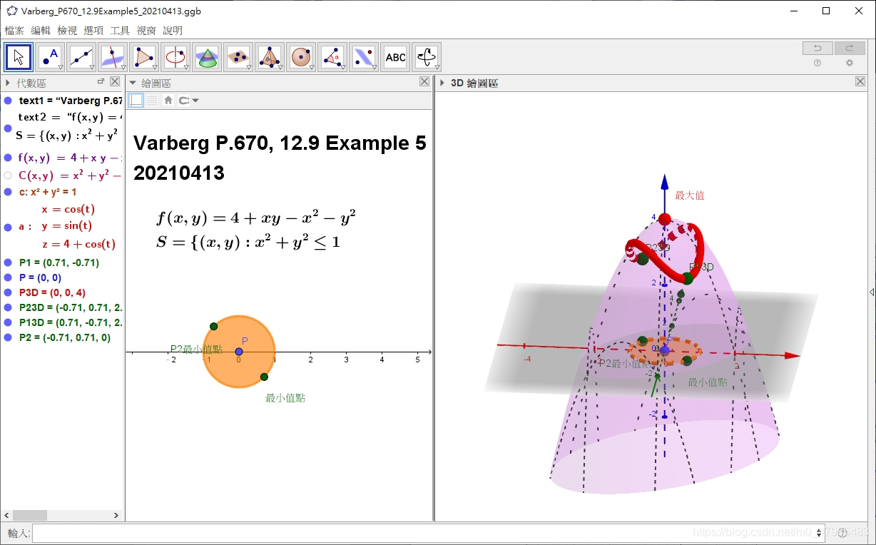 可以按右鍵, 轉動視角, 同樣的效果, 如果僅是靜態圖, 用 pyplot, 恐怕要手忙腳亂一陣子, 3D 可能還要動用到 MayaView 等, 如果是動畫, 還得查一下 Tkinter 的指令等.
另一方面, 如果完全用 GeoGebra 算微積分, 因為 GeGebra 主力是動態幾何, 會覺得指令不夠, 要想有完整的微積分, 最佳化, 矩陣, 解微分方程等函數, 還是要搭配依賴較完整的程式語言, 例如 Python+SciPy(先載入NumPy)+SymPy, 或 Matlab, Maple, Mathematica , 或 R, Maxima 等.
所以我自己的建議是可以兩方搭配一起用, 當然學習的時間, 以我本人的經驗, 教師以課餘瑣碎的時間邊教邊摸索自學, 約需1~3年的時間(有熟悉的人帶領學習的前提下, GeoGebra只需2,3個月, 自己摸索可能要半年才能製作較進階的GeoGebra內容, 另外 Python+NumPy+SciPy+SymPy 如果有人教或有跟隨課程應該半年就可以基本夠用了).
| 微積分軟體之建議搭配 | 是否免費 | 動態幾何(滑鼠+微積分指令+3D) | 程式語言 | 數值與符號運算功能 |
|---|---|---|---|---|
| 皆是 | GeoGebra | Python+SciPy(先載入NumPy)+SymPy | 皆有 | |
| 皆是 | GeoGebra | R | 數值與統計運算較強 | |
| 皆是 | GeoGebra | GNU Octave | 數值運算較強(指令類似Matlab) | |
| 皆是 | GeoGebra | Maxima | 符號運算較強 | |
| 一半 | GeoGebra | Matlab | 數值運算較強 | |
| 一半 | GeoGebra | Maple | 符號運算較強 | |
| 一半 | GeoGebra | Mathematica | 符號運算較強 | |
| 註 | 皆是 | desmos | desmos 與 GeoGebra 的繪圖計算器非常類似, 雖然簡易上手, 但是不像GeoGebra功能較全面性 |
大家可以看的出來, 初學者乾脆選第一項: GeoGebra 搭配 Python(+SciPy(先載入NumPy)+SymPy), 既免費開源, 又數值計算與符號運算功能一次到位, 不過學習過程較長, 不像商用軟體, 所有指令都一次到位, Python(+SciPy(先載入NumPy)+SymPy) 需多花時間熟悉, 那些指令是 Python 內建的, 那些在 scipy, 那些在 sympy, 算是一個小的困擾. 作者用過 Maple 多年, Maple是以符號運算知名, 深知, 符號運算較強的軟體在數值運算遠不如Matlab 之指令豐富與效能快速, 作者也用過 Matlab 多年, , Matlab 是以矩陣數值運算知名, 深知, 數值運算較強的軟體在符號運算遠不如 Maple之指令豐富,
而偏偏, 微積分計算的特質, 就是混合數值計算與符號運算才能完整, 以作者教學的經驗, 在大一微積分範圍, 可以只用符號運算強的軟體就很夠用, 甚至只有 GeoGebra也很夠了, 故如果 初學者選 GeoGebra 搭配 符號運算強的軟體 Maxima, Maple, Mathematica 等, 或數值計算強的軟體 Matlab, Octave 等都可以. 但是如果考量後續的延伸性, 延伸到數學系大二大三的數值計算, 科學計算, 數學建模, 資料分析等, 工程學系的高等工程數學, 運籌學系的 單純形法, 動態規劃法, 非線性規劃等等, 選擇搭配符號運算強的軟體會開始感到效能不濟, 尤其在跑一些尺度稍大的演算法時, 就會走上作者的同樣的路, 先學 Maple, 之後必須再學 Matlab 才夠用. 故如果考量後續的延伸大二以上到研究所, 建議初學者選擇 GeoGebra 搭配數值計算強的軟體, 當然如果一開始就選 GeoGebra 搭配 Python(+SciPy(先載入NumPy)+SymPy), 既免費開源, 又數值計算與符號運算功能一次到位, 就不用煩惱這些.
| 微積分或後續科學計算軟體之建議搭配 | 是否免費 | 大一大二微積分範圍 | 延伸至大二以上的科學計算,非線性規劃,高等工程數學等 | 數值與符號運算功能 |
|---|---|---|---|---|
| 皆是 | GeoGebra+ Python+SciPy(先載入NumPy)+SymPy | GeoGebra+ Python+SciPy(先載入NumPy)+SymPy | 皆有 | |
| Octave, C, Java 是 | GeoGebra+數值計算強的軟體 Matlab, Octave R, C, Java 等 | GeoGebra+數值計算強的軟體 Matlab, Octave, R, C, Java 等 | 數值運算較強 | |
| Maxima是 | GeoGebra+符號運算強的軟體 Maxima, Maple, Mathematica 等 | 大尺度數值模擬較耗時 | 符號運算較強 | |
| 是 | GeoGebra | 數值與符號運算功能皆夠大一大二用 |
desmos 與 GeoGebra 的比較
近幾年網路似乎開始鼓吹 desmos 一款類似 GeoGebra 的軟體, 較簡易上手, 但是我發現功能相當受限, 介面與 GeoGebra 的繪圖計算器類似, 不知是誰學誰的? 兩個都可以畫 3D 函數圖.
跟 GeoGebra 比起來, desmos 的功能只是 GeGebra的一小部分, 但是 desmos 似乎較會做宣傳.
以下是 GeoGebra官網線上 的繪圖計算器, 可以把他想成是 GeoGebra 6 的一個特例的介面狀況 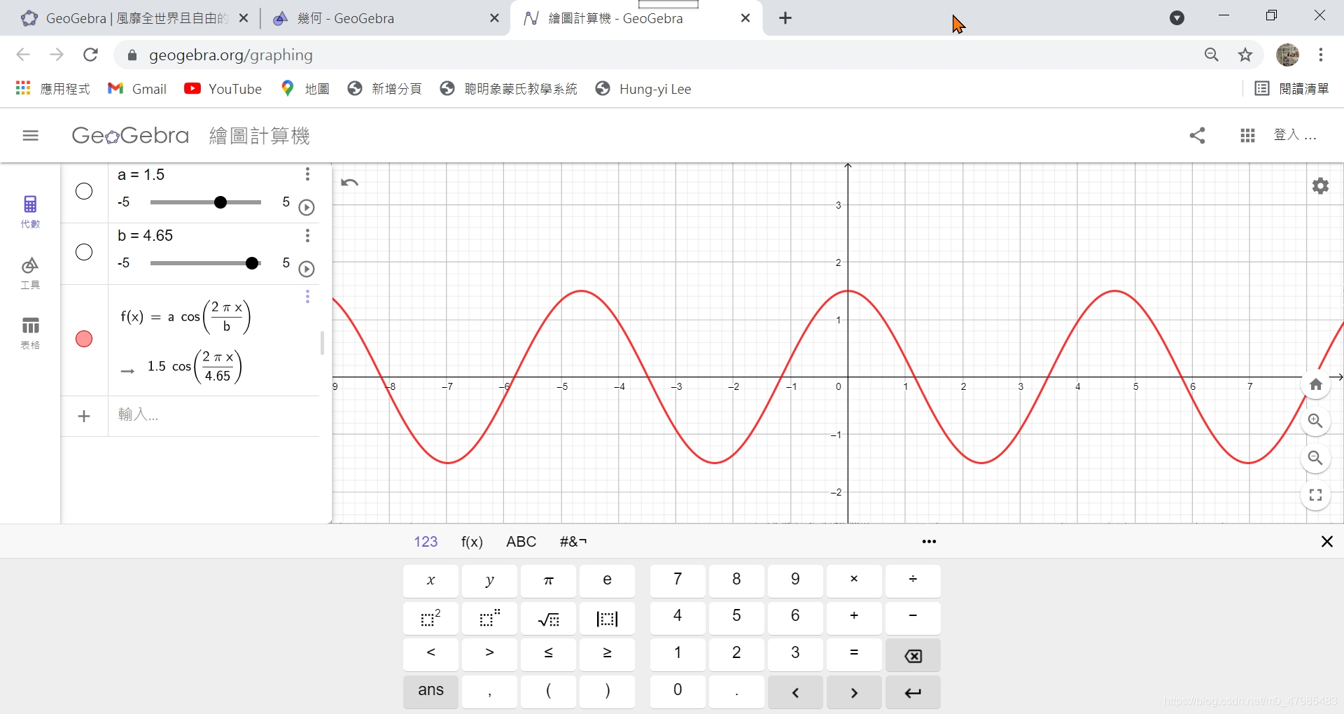
以下是 desmos 官網線上 的介面, 與 GeoGebra 官網 的線上繪圖計算器非常類似:
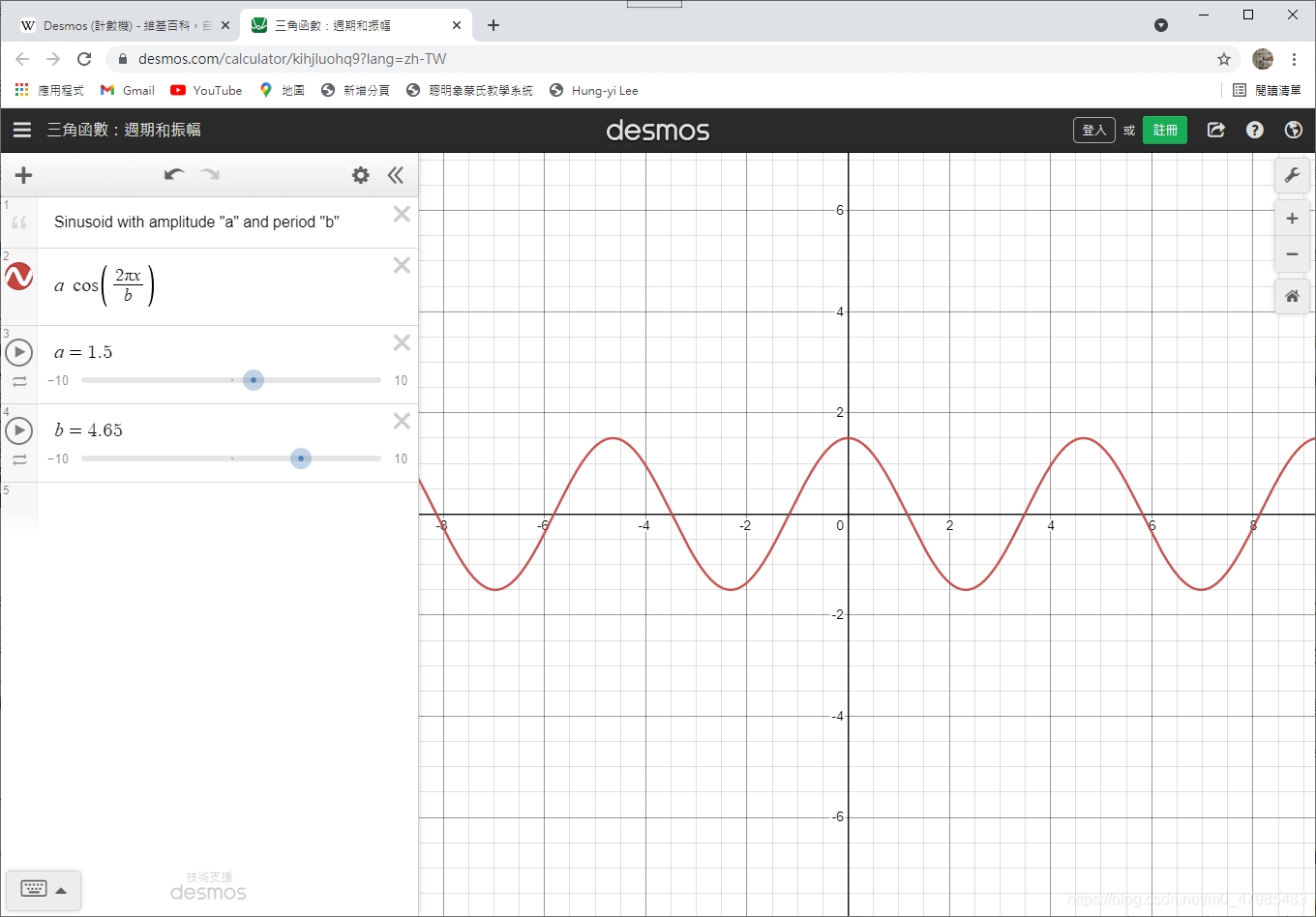
Python 中有數學指令的模組或程式庫
以下大略介紹 Python 中有數學指令的模組或程式庫, 部分參考自 陳擎文教學網, https://acupun.site/lecture/python_math/index.htm#chp5 link
| Python 中有數學指令的模組或程式庫 | 內建模組或外部程式庫 | 包含內容 | 大一大二微積分範圍 | 延伸至大二以上的科學計算,非線性規劃,高等工程數學等 | 數值與符號運算功能 |
|---|---|---|---|---|---|
| 內建(原生) math 模組 | 基本數學函數與指令: pi, e, sqrt(x) , fabs(x), factorial(x), fmod(x,y), sin(x), sinh(x), cos(x), tan(x)等 | 不足應付 | 不足應付 | 數值運算 | |
| 內建(原生 cmath | 處理複數運算 | 不足應付 | 不足應付 | 數值運算 | |
| 矩陣運算 NumPy 外部程式庫 | NumPy 支援高維度, 大尺度矩陣(即array)運算,此外也針對矩陣運算提供大量的數學函式函式庫。在矩陣計算範圍內, NumPy 提供了與 MATLAB 相似的功能與操作方式 | 不適合 (較適合線性代數課程) | 支援高維度矩陣運算 | 數值運算 | |
| 數值運算 SciPy (底層含 NumPy) 外部程式庫 | SciPy 包含的模組有最佳化、線性代數、積分、插值、特殊函數、快速傅立葉變換、訊號處理和圖像處理、常微分方程式求解和其他科學與工程中常用的計算。 與其功能相類似的軟體還有MATLAB、GNU Octave和Scilab。 | 足夠應付微積分數值計算部分 | 足夠應付數值運算部分 | 數值運算 | |
| 符號運算 SymPy 外部程式庫 | Sympy是一個數學符號庫(sym代表了symbol,符號),包括了積分,微分方程,三角等各種數學運算方法,是工科最基本的數學函數庫,用起來媲美Matlab, Maple,而且其精度比math函數庫精確。 例如: 多項式的合併、展開、化簡 微積分運算 微分方程求解 線性代數運算 係數匹配 繪圖 進階:SymPy 可以支援的內容包括但不限於: 1. 範疇論(Category Theory); 2. 微分幾何(Differential Geometry); 3. 常微分方程(ODE); 4. 偏微分方程(PDE); 5. 傅立葉轉換(Fourier Transform); 6. 集合論(Set Theory); 7. 邏輯計算(Logic Theory)。 | 足夠應付 | 足夠應付所有符號運算與小尺度數值運算部分 | 符號運算與部分數值運算 |
Python 中執行微積分的符號運算的主力是 SymPy
特別指出, 經過作者在網路搜尋, 發現, 一般在網路講解用 Python 算微積分的網誌或課程, 主要還是用 SymPy 來做各種微積分的計算, SymPy 是提供求符號計算的 程式庫, 類似 Maple, Mathematica 等, 但是不像Maple, Mathematica是需付費的, SymPy是開源免費,只需在 Python 裝好之後再加裝第三方程式庫進來就好, 如果是使用 Anaconda 或 Google的 CoLab, 則都會已經自動裝好. (Matlab 裡 搭配符號計算的引擎是 MuPad, 最一開始是用 Maple引擎, 不知何原因後來改成用Mupad).
Python 可以執行 calculus 的 程式庫:
- scipy: 可以提供求
數值的微分, 數值的積分, 零根, min, max, 解 ODE 等數值計算, scipy 已包含 NumPy 在內. - sympy: 可以提供求符號計算的 微分, 積分, Taylor series, 零根, min, max, 解 ODE 等符號計算, 當然數值計算也能, 在單單微積分範圍內, sympy的指令還是較齊全!, 但是學習符號計算通常較困難, 需要較多的數學素養.
對於學生, 如果只需要計算數值解的 微分, 積分, 求零根, 極大極小值(min, max), 解常微分方程ODE等等, 可以只學 SciPy 即可, SymPy 的學習曲線較陡峭.
數值計算與符號計算之差別
所謂 數值微分 numerical differentiation、數值積分 numerical integration, 是求其近似值, 而非公式. 例如以下 cos(x) 的數值積分是求其近似值, 而非公式: \(\int_0^{1.2} cos(x) dx = 0.9320390859672262\)
>>> from scipy import integrate

>>> integrate.quad(scipy.cos,0,1.2)
(0.9320390859672262, 1.0347712530914001e-14)
相對於此是==符號計算 symbolic computation== 的微分或積分, 也就是我們大學用手算的微分或積分的解析解, 有明確的數學式子的解答, (注意, 不是所有的積分都有解析解, 例如橢圓積分, 或是例如 $\int sin(x^2) dx$ 等, 都沒有明確的解析式子 的表法, 對於這類的積分, 只能求近似解(數值解), 或是用特殊函數表達其解),
符號計算 是求公式, 例如以下 cos(x) 的手算積分是求公式而非近似值: \(\int cos(x) dx = sin(x) +C\)
也就是 ==符號計算 相當於叫電腦模擬我們中學或大學時用手算出數學公式的計算==
以下是 SymPy 的語法
>>> import sympy
>>> x = sympy.Symbol('x')
>>> x
x
>>> sympy.integrate( sympy.cos(x), x)
sin(x)
>>> sympy.diff( sympy.cos(x), x)
-sin(x)
註: math 模組與 numpy 都沒數值微分、數值積分的指令, numpy.diff() 是求 array差值. Python 中似乎缺乏數值微分的指令, 通常都是用 sympy 來算微分, scipy 似乎也只有數值積分, 讀者可以自己寫一個求數值微分的函數, codes 可以參考後面 數值微分那節.
以下陳擎文教授此站主要介紹使用 sympy 算微積分的課程講義: 陳擎文教學網:python求解數學式(高中數學,大學數學,工程數學,微積分) 方程式,多項式,函數,三角函數,微分,積分,泰勒級數,傅立葉級數,傅立葉積分,傅立葉轉換,一階微分方程式,二階微分方程式,三階微分方程式,偏微分方程式,聯立方程式矩陣解法,張量,向量的坐標轉換, 複數,極坐標 https://acupun.site/lecture/python_math/index.htm#chp5 link
Python, NumPy, SciPy, SymPy 的安裝或線上使用
安裝Python 請參考本人的另一篇 https://blog.csdn.net/m0_47985483/article/details/109522800 安裝Python 那節 link
安裝 NumPy, SciPy, Matplotlib, Pandas Python安裝之後並沒有 NumPy, SciPy, Matplotlib, Pandas, 他們是額外加裝在 Python 上的程式庫, 在 Windows 下, 打開 “命令提示字元” 的視窗, 輸入
>> pip install numpy >> pip install scipy >> pip install sympy
或是使用 Anaconda, 安裝好之後, 最重要的程式庫都已裝好, Anaconda + Jupyter Notebook 會自動安裝好所需的科學計算或大數據的程式庫 (or Anaconda + Spyder or Anaconda + PyCharm 等),
線上使用可以用 Google Colab, 也會自動安裝好所需的科學計算或大數據的程式庫.
Python 中執行數值計算的主力是 SciPy (需先載入NumPy)
SciPy 的底層是 NumPy. scipy 的入門說明講義不太好找, 常常會搜尋到別的頁面, 在 https://scipy-lectures.org/index.html這裡, link
SciPy的模組種類
https://docs.scipy.org/doc/scipy/reference/index.html
scipy的模組很多, 本篇只關注跟微積分較相關的兩個 Integration and ODEs (scipy.integrate) Optimization and root finding (scipy.optimize)
API Reference The exact API of all functions and classes, as given by the docstrings. The API documents expected types and allowed features for all functions, and all parameters available for the algorithms.
Clustering package (scipy.cluster) Constants (scipy.constants) Discrete Fourier transforms (scipy.fft) Legacy discrete Fourier transforms (scipy.fftpack) Integration and ODEs (scipy.integrate) Interpolation (scipy.interpolate) Input and output (scipy.io) Linear algebra (scipy.linalg) Miscellaneous routines (scipy.misc) Multidimensional image processing (scipy.ndimage) Orthogonal distance regression (scipy.odr) Optimization and root finding (scipy.optimize) Signal processing (scipy.signal) Sparse matrices (scipy.sparse) Sparse linear algebra (scipy.sparse.linalg) Compressed sparse graph routines (scipy.sparse.csgraph) Spatial algorithms and data structures (scipy.spatial) Special functions (scipy.special) Statistical functions (scipy.stats) Statistical functions for masked arrays (scipy.stats.mstats) Low-level callback functions
sciPy 求零根
1.6.5.3. Finding the roots of a scalar function
ref: https://scipy-lectures.org/intro/scipy.html#finding-the-roots-of-a-scalar-function link
用 scipy.optimize.root(fun, ,,)求零根
scipy.optimize.root(fun, x0, args=(), method=’hybr’, jac=None, tol=None, callback=None, options=None)
官網的例子 \(f(x) = x^2 + 10\sin(x)\) 求其零根.
import numpy as np
from scipy import optimize
import matplotlib.pyplot as plt

def f(x):
    return x**2 + 10*np.sin(x)

x = np.arange(-10, 10, 0.1)

plt.plot(x, f(x))

root = optimize.root(f, x0=1)
print(root)
print('root1=', root.x)

root2 = optimize.root(f, x0=-2.5)
print('root2=', root2.x)
輸出:
>>>
= RESTART: C:\Users\user\Desktop\1.6.5.3. Finding the roots of a scalar function.py
    fjac: array([[-1.]])
     fun: array([0.])
 message: 'The solution converged.'
    nfev: 10
     qtf: array([1.33310463e-32])
       r: array([-10.])
  status: 1
 success: True
       x: array([0.])
root1= [0.]
root2= [-2.47948183]
SciPy 求數值微分、數值積分
所謂 數值微分 numerical differentiation、數值積分 numerical integration, 是求其近似值, 相對於此, 是符號計算 symbolic computation 的微分或積分, 也就是我們大學用手算的微分或積分的解析解, 有明確的數學式子的解答.
數值微分
math 模組與 numpy 都沒數值微分、數值積分的指令, numpy.diff 是求 array差值. Python 模組與程式庫中似乎缺乏數值微分的指令, 通常都是用 sympy 來算微分, scipy 似乎只有數值積分, 數值微分的原理很簡單, 照定義算, 取極限的意思, 就是切夠小格就好, 可以自己寫一個求數值微分的函數.
Ex: 自己寫一個求數值微分的函數. Sol: 自己寫一個求數值微分的函數 並不需要用到 scipy, 只需用 Python 或至多 numpy, 根據微分的定義: \(f'(x_0) = \lim_{ \nabla x \rightarrow 0 } \frac{f(x_0+\nabla x) - f(x_0)}{\nabla x}\) 故只要用夠小的 $\nabla x$ 去計算 \(\frac{f(x_0+\nabla x) - f(x_0)}{\nabla x}\) 就是 $f’(x_0)$ 的近似值.
以下自定義函數 numericalDiff(f, x_0, n)
輸入引數中的 f, 為求微分之函數, 可以用 lambda 表達式 輸入, x_0 為求微分之點, n, 代表切 1/n 這麼小, i.e., $\nabla x = 1/n$, 如果要精度較高, 可以輸入較大的 n, 例如 10000, 代表 $\nabla x = \frac{1}{10000}=0.0001$.
lambda 表達式 : 例如 lambda x: x**2 代表一個臨時產生的函數 $f(x) = x^2$.
import math lambda x: math.sin(x**2) (注意: sin(x) 需要使用內建的 math 模組) 代表一個臨時產生的函數 $f(x) = sin(x^2)$.
>>> import math
>>> f = lambda x: math.sin(x**2)
>>> f(2)
-0.7568024953079282
自定義數值微分的函數 numericalDiff() 如下方 codes, 呼叫此函數之用法, 示例: numericalDiff( lambda x: x**2, 1, 100) 代表對 函數 $f(x) = x^2$ 求微分, 在 x=1 的位置, $\nabla x$ 取為 $\frac{1}{100}=0.01$. 如果要精度較高, 可以輸入較大的 n, 例如 n=10000, 代表 $\nabla x = \frac{1}{10000}=0.0001$,
自定義數值微分的函數 numericalDiff() 的程式碼:
# By Prof. P-J Lai MATH NKNU 20210605
# Numerical differentiation
# numericalDiff.py

def numericalDiff(f, x_0, n):
    deltaX = 1/n
    #print( 'the Df of x^2 at {} is {}'.format(x_0, (f(x_0+deltaX) - f(x_0))/deltaX)  )
    print( f'the Df of x^2 at {x_0} is { (f(x_0+deltaX) - f(x_0))/deltaX }' )

    return (f(x_0+deltaX) - f(x_0))/deltaX

numericalDiff( lambda x: x**2, 1, 100)
輸出:
>>>
================ RESTART: C:/Users/user/Desktop/numericalDiff.py ===============
the Df of x^2 at 1 is 2.0100000000000007
數值積分
當我們想要用 scipy 算數值積分時, 需先下 from scipy import integrate, 載入 scipy 之 integrate 模組, (或使用 from scipy import * 載入所有指令) 不能只載入 scipy, 再直接使用 scipy.integrate.quad(), 例如以下
>>> import scipy
>>> scipy.integrate.quad(scipy.cos,0,1.2)
Traceback (most recent call last):
  File "<pyshell#1>", line 1, in <module>
    scipy.integrate.quad(scipy.cos,0,1.2)
AttributeError: module 'scipy' has no attribute 'integrate'
以下才正確 先下 from scipy import integrate 再呼叫 integrate.quad(scipy.cos,0,1.2),
>>> from scipy import integrate

>>> integrate.quad(scipy.cos,0,1.2)
(0.9320390859672262, 1.0347712530914001e-14)
或 scipy.integrate.quad(scipy.cos,0,1.2) 皆可
>>> from scipy import integrate
>>> scipy.integrate.quad(scipy.cos,0,1.2)
(0.9320390859672262, 1.0347712530914001e-14)
查詢 scipy.integrate 中的積分指令
>>> from scipy import integrate
>>> dir(scipy.integrate)
Traceback (most recent call last):
  File "<pyshell#10>", line 1, in <module>
    dir(scipy.integrate)
NameError: name 'scipy' is not defined
>>> dir(integrate)
['AccuracyWarning', 'BDF', 'DOP853', 'DenseOutput', 'IntegrationWarning', 'LSODA', 'OdeSolution', 'OdeSolver',
'RK23', 'RK45', 'Radau',
'__all__', '__builtins__', '__cached__',
'__doc__', '__file__', '__loader__', '__name__', '__package__', '__path__', '__spec__', '_bvp', '_dop', '_ivp',
'_ode', '_odepack', '_quad_vec', '_quadpack', '_quadrature', 'complex_ode', 'cumtrapz', 'cumulative_trapezoid',
'dblquad', 'fixed_quad', 'lsoda', 'newton_cotes', 'nquad', 'ode', 'odeint', 'odepack', 'quad', 'quad_explain',
'quad_vec', 'quadpack', 'quadrature', 'romb', 'romberg', 'simps', 'simpson', 'solve_bvp', 'solve_ivp',
'test', 'tplquad', 'trapezoid', 'trapz', 'vode']
官網 1.6.7.1. Function integrals 之例子
求
\[\int_0^{\frac{\pi}{2}} sin(x) dx \sim 1\]res, err = quad(np.sin, 0, np.pi/2) res 是輸出之 結果, err 是誤差, np.allclose(res, 1) 是詢問 res 與理論值 1 是否接近? (註: math.isclose(a, b) 功能類似)
>>> from scipy.integrate import quad
>>> import numpy as np
>>> res, err = quad(np.sin, 0, np.pi/2)
>>>> res
0.9999999999999999
>>> err
1.1102230246251564e-14
>>> np.allclose(res, 1)
True
>>> np.allclose(err, 1 - res)
True
>>>
1.6.5 Optimization and fit 求極值與曲線擬合(內外插法)
Ref: Scipy Lecture Notes, 1.6.5 Optimization and fit: scipy.optimize, link
params, params_covariance = optimize.curve_fit(test_func, x_data, y_data, p0=[2,2])
#!/usr/bin/env python
# coding: utf-8

# # 6.5 Optimization and fit: scipy.optimize
# Ref: Scipy Lecture Notes — Scipy lecture notes主頁2020

# In[3]:


from scipy import optimize
import numpy as np


# In[4]:


x_data = np.linspace(-5,5, num=50)


# In[5]:


x_data


# In[6]:


y_data = 2.9*np.sin(1.5*x_data) + np.random.normal(size=50)


# In[7]:


y_data


# In[8]:


def test_func(x, a, b):
    return a*np.sin(b*x)


# In[9]:


params, params_covariance = optimize.curve_fit(test_func, x_data, y_data, p0=[2,2])


# In[10]:


print(params)
##output
##>>>
##= RESTART: C:\data\NEW\網路免費軟體資料\Python教學\Python科學計算\
## sci_optimize_求##min_max_zeros_求零根可以轉成求min\
## 6.5 Optimization and fit scipy.optimize.py
##[2.97083835 1.52207958]


# In[11]:


import matplotlib.pyplot as plt


# In[24]:


plt.figure(figsize=(10,4))
plt.scatter(x_data, y_data, label='data')
x=np.linspace(-5,5, num=50)
y=test_func(x,params[0],params[1])
plt.plot(x,y,color='red', label='optimize.curve_fit')
plt.legend()
plt.show()


# In[ ]:
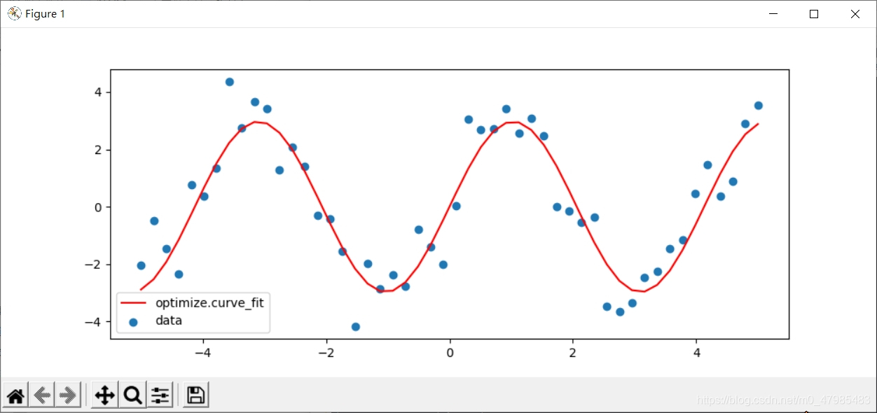
(1.6.5) 2.7 scipy.optimize 求極值
scipy 的 optimizer種類: scipy.optimize 基本上是求極植(max, min), 至於求零根, 不管事純量函數 scalar function 或 向量值函數 vector-valued function 都可以將求零根問題
\(F(x)=(f_1(x), f_2(x),\cdots,f_n(x))=0,\) 轉為求min 的問題 \(\min \left(\sum_{i=1}^n f_i(x)^2 \right).\)
以下是scipy.optimize 中各種可以使用的求極植的方法(函數), 參考自 Ref: Scipy Lecture Notes, 1.6.5 Optimization and fit: scipy.optimize, link 2.7. Mathematical optimization: finding minima of functions, link 20210603 online.
這裡有簡單總結何種情況使用何種 optimizer 求解器:
2.7.5. Practical guide to optimization with scipy 2.7.5.1. Choosing a method 選擇適合的 optimizer 求解器 link
result = optimize.minimize_scalar(f)
optimize.minimize(f, [2, -1], method="CG")
optimize.minimize(f, [2,-1], method="Newton-CG", jac=jacobian)
result = optimize.minimize(g, [1, 1], method="Powell", tol=1e-10)

optimize.minimize(f, np.array([0, 0]), method="SLSQP",
constraints={"fun": constraint, "type": "ineq"})

result = optimize.minimize_scalar(f, bracket=(-5, 2.9, 4.5), method="Brent",
options={"maxiter": iter}, tol=np.finfo(1.).eps)

optimize.minimize(f, np.array([0, 0]), method="L-BFGS-B",
bounds=((-1.5, 1.5), (-1.5, 1.5)))

optimize.minimize(f, [2, -1], method="Nelder-Mead")

optimize.brute(f, ((-1, 2), (-1, 2)))

optimize.minimize(f, np.array([0, 0]), bounds=((-1.5, 1.5), (-1.5, 1.5)))

optimize.minimize(f, x0, constraints={"fun": constraint, "type": "ineq"})
2.7.5.1. Choosing a method All methods are exposed as the method argument of scipy.optimize.minimize().
Without knowledge of the gradient • In general, prefer BFGS or L-BFGS, even if you have to approximate numerically gradients. These are also the default if you omit the parameter method - depending if the problem has constraints or bounds • On well-conditioned problems, Powell and Nelder-Mead, both gradient-free methods, work well in high dimension, but they collapse for ill-conditioned problems. With knowledge of the gradient • BFGS or L-BFGS. • Computational overhead of BFGS is larger than that L-BFGS, itself larger than that of conjugate gradient. On the other side, BFGS usually needs less function evaluations than CG. Thus conjugate gradient method is better than BFGS at optimizing computationally cheap functions. With the Hessian • If you can compute the Hessian, prefer the Newton method (Newton-CG or TCG). If you have noisy measurements • Use Nelder-Mead or Powell.
scipy 的 constants 模組
ref: http://yhhuang1966.blogspot.com/2020/04/python-scipy.html link
scipy 的 constants 必須先 import
只有 sci.pi, sci.e 等是 scipy 內建的, 其餘常數都必須先 from scipy import constants 才能叫出 constants下的常數 golden, c等
>>>import scipy
>>> scipy.pi
3.141592653589793
>>> scipy.c
Traceback (most recent call last):
  File "<pyshell#10>", line 1, in <module>
    scipy.c
AttributeError: module 'scipy' has no attribute 'c'
>>> scipy.golden
Traceback (most recent call last):
  File "<pyshell#11>", line 1, in <module>
    scipy.golden
AttributeError: module 'scipy' has no attribute 'golden'
>>> scipy.e
2.718281828459045
如果已載入scipy, 想直接用 scipy.constants.golden 是不行的 必須特別單獨載入 constants, from scipy import constants 才看的到 constants 的屬性, 也才能用 dir(constants)
以下是錯誤的
>>>import scipy
>>> scipy.constants.golden
Traceback (most recent call last):
  File "<pyshell#1>", line 1, in <module>
    scipy.constants.golden
AttributeError: module 'scipy' has no attribute 'constants'

>>> dir(scipy.constants)
Traceback (most recent call last):
  File "<pyshell#2>", line 1, in <module>
    dir(scipy.constants)
AttributeError: module 'scipy' has no attribute 'constants'
>>> dir(constants)
Traceback (most recent call last):
  File "<pyshell#3>", line 1, in <module>
    dir(constants)
NameError: name 'constants' is not defined
以下是正確的
>>> from scipy import constants
>>> dir(constants)
['Avogadro', 'Boltzmann', 'Btu', 'Btu_IT', 'Btu_th', 'ConstantWarning', 'G', 'Julian_year', 'N_A', 'Planck', 'R', 'Rydberg', 'Stefan_Boltzmann',
'Wien', '__all__', '__builtins__', '__cached__', '__doc__', '__file__', '__loader__', '__name__', '__package__', '__path__', '__spec__',
'_obsolete_constants', 'acre', 'alpha', 'angstrom', 'arcmin', 'arcminute', 'arcsec', 'arcsecond', 'astronomical_unit', 'atm', 'atmosphere',
 'atomic_mass', 'atto', 'au', 'bar', 'barrel', 'bbl', 'blob', 'c', 'calorie', 'calorie_IT', 'calorie_th', 'carat', 'centi', 'codata', 'constants',
 'convert_temperature', 'day', 'deci', 'degree', 'degree_Fahrenheit', 'deka', 'dyn', 'dyne', 'e', 'eV', 'electron_mass', 'electron_volt',
 'elementary_charge', 'epsilon_0',
 'erg', 'exa', 'exbi', 'femto', 'fermi', 'find', 'fine_structure', 'fluid_ounce', 'fluid_ounce_US',
 'fluid_ounce_imp', 'foot', 'g', 'gallon', 'gallon_US', 'gallon_imp', 'gas_constant', 'gibi', 'giga', 'golden', 'golden_ratio',
 'grain', 'gram', 'gravitational_constant',
 'h', 'hbar', 'hectare', 'hecto', 'horsepower', 'hour', 'hp', 'inch', 'k', 'kgf', 'kibi', 'kilo', 'kilogram_force',
 'kmh', 'knot', 'lambda2nu', 'lb', 'lbf', 'light_year', 'liter', 'litre', 'long_ton', 'm_e', 'm_n', 'm_p', 'm_u', 'mach', 'mebi', 'mega',
 'metric_ton', 'micro', 'micron', 'mil', 'mile', 'milli', 'minute', 'mmHg', 'mph', 'mu_0', 'nano', 'nautical_mile', 'neutron_mass',
 'nu2lambda', 'ounce', 'oz', 'parsec', 'pebi', 'peta', 'physical_constants', 'pi', 'pico', 'point', 'pound', 'pound_force', 'precision',
 'proton_mass', 'psi', 'pt', 'short_ton', 'sigma', 'slinch', 'slug', 'speed_of_light', 'speed_of_sound', 'stone', 'survey_foot',
 'survey_mile', 'tebi', 'tera', 'test', 'ton_TNT', 'torr', 'troy_ounce', 'troy_pound', 'u', 'unit', 'value', 'week', 'yard', 'year',
 'yobi', 'yotta', 'zebi', 'zepto', 'zero_Celsius', 'zetta']

>>> constants.c
299792458.0
>>> constants.golden
1.618033988749895
SymPy
從 SymPy 的模組可以看出 SymPy 主要還是在數學的深度與廣度的設計, 主力還是在數學範圍, 底下有較深的數學主題, 例如 李群 Lie algebra, 範疇論Category Theory, 密碼學Cryptography, 偏微分方程 PDE, 張量 tensor 等等, 用這來教微積分, 應該是綽綽有餘, 但是對於高效能的數值算法, 她並不擅長, 還是要用 SciPy 或 Matlab 等輔助.
Ref: SymPy 的模組可以在此查看: SymPy Modules Reference, https://docs.sympy.org/latest/modules/index.html link
SymPy 的模組很多
Algebras Introduction Quaternion Reference Assumptions Calculus Category Theory Combinatorics Cryptography Diophantine Discrete Geometry Inequality Solvers Lie Algebra Logic Matrix Expressions Number Theory ODE PDE Physics Plotting Sets Simplify Solvers Stats Tensor Vector 等等
官網操作手冊
官網手冊 目前 2021 的 1.8 版 , 跟比 2018 的 1.3 版比, 就多了 7百多頁, 更新的速度相當驚人! Ref: Welcome to SymPy’s documentation!, https://docs.sympy.org/latest/index.html link
2.2.1 What is Symbolic Computation 求 $\sqrt{8}$
Symbolic computation deals with the computation of mathematical objects symbolically. This means that the mathematical objects are represented exactly, not approximately, and mathematical expressions with unevaluated variables are left in symbolic form.
官網文件先舉 開更號的例子, 在 Python 中我們要算 $\sqrt{9}$, 算出來的是浮點數
>>> 9**(1/2)
3.0
或是用 math.sqrt()
>>> import math
>>> math.sqrt(9)
3.0
此時可以使用符號運算的功能, 來保持手寫數學式子的呈現,
>>> sympy.sqrt(5)
sqrt(5)
如果覺得 sqrt(5) 不像手寫的風格, 可以使用 sympy.pprint()美化列印, 印出為一如我們平時手寫數學式子的風格
>>> sympy.pprint(sympy.sqrt(5))
√5
此時 sympy不會立即傳回浮點值, 而是保持在一個數學符號 $\sqrt{5}$ 的’狀態 但是碰到再對他平方, 還是能夠算出為 5, 而不是一個類似字串的死符號,
>>> sympy.sqrt(5)**2
5
另一種好處是, 例如碰到 $\sqrt{8}$, 他會回我們手寫計算的習慣呈現方式 $2\sqrt{2}$
>>> sympy.sqrt(8)
2*sqrt(2)
>>> sympy.pprint(sympy.sqrt(8))
2⋅√2
另外一種情況是, 如果我們想呈現 $(\sqrt{5})^2$ 這樣的寫法, 又希望他同時能對其做相對的數學運算 如果用以上的指令, 會立刻傳回浮點值
>>> (math.sqrt(5))**2
5.000000000000001
可以使用延遲求值的方式, (Prevent expression evaluation, Ref: Advanced Expression Manipulation, https://docs.sympy.org/latest/tutorial/manipulation.html#prevent-expression-evaluation link) 這種方式在 Maple 裡 或是一般的符號運算軟體裡也常用
一種方法是可以用 sympy.UnevaluatedExpr(sympy.sqrt(5)) 將他包裹起來
>>> expSqrt5 = sympy.UnevaluatedExpr(sympy.sqrt(5))
>>> expSqrt5
sqrt(5)
之後再對他平方, 也不會展開為 5:
>>> expSqrt5**2
(sqrt(5))**2
>>> sympy.pprint(expSqrt5**2)
  2
√5
如果要求值, 可以先用 doit(), 解除 延遲求值
>>> expSqrt5**2.doit()
SyntaxError: invalid syntax
>>> (expSqrt5**2).doit()
5
再用 evalf()
>>> expSqrt5.doit().evalf()
2.23606797749979
另一種 延遲求值 方法是, sympy.sqrt(5,evaluate=False)
>>> sympy.sqrt(5,evaluate=False)
sqrt(5)
但是再對他平方, 會展開為 5
>> expSqrt5_1=sympy.sqrt(5,evaluate=False)
>>> expSqrt5_1
sqrt(5)
>>> expSqrt5_1**2
5
import sympy
x, y=sympy.symbols('x, y')
x, y=sympy.symbols('x y')
x,y
(x, y)
type(x)
sympy.core.symbol.Symbol
foo=x+2*y
foo
$\displaystyle x + 2 y$
type(foo)
sympy.core.add.Add
foo+1
$\displaystyle x + 2 y + 1$
foo-y
$\displaystyle x + y$
x*foo
$\displaystyle x \left(x + 2 y\right)$
(x*foo).expand()
$\displaystyle x^{2} + 2 x y$
expandFoox = sympy.expand(x*foo)
expandFoox
$\displaystyle x^{2} + 2 x y$
sympy.factor(expandFoox)
$\displaystyle x \left(x + 2 y\right)$
2.2.3 The Power of Symbolic Computation
expr = sympy.sin(x**2)*sympy.exp(2*x)
expr
$\displaystyle e^{2 x} \sin{\left(x^{2} \right)}$
DiffExpr = sympy.diff(expr)
DiffExpr
$\displaystyle 2 x e^{2 x} \cos{\left(x^{2} \right)} + 2 e^{2 x} \sin{\left(x^{2} \right)}$
sympy.integrate(DiffExpr,x)
$\displaystyle 2 \left(\int e^{2 x} \sin{\left(x^{2} \right)}\, dx + \int x e^{2 x} \cos{\left(x^{2} \right)}\, dx\right)$
expr1 = sympy.sin(x)*sympy.exp(x)
expr1
$\displaystyle e^{x} \sin{\left(x \right)}$
DiffExpr1 = sympy.diff(expr1,x)
DiffExpr1
$\displaystyle e^{x} \sin{\left(x \right)} + e^{x} \cos{\left(x \right)}$
sympy.integrate(DiffExpr1)
$\displaystyle e^{x} \sin{\left(x \right)}$
sympy.integrate(sympy.sin(x**2),x)
$\displaystyle \frac{3 \sqrt{2} \sqrt{\pi} S\left(\frac{\sqrt{2} x}{\sqrt{\pi}}\right) \Gamma\left(\frac{3}{4}\right)}{8 \Gamma\left(\frac{7}{4}\right)}$
sympy.integrate(sympy.sin(x**2),(x, -sympy.oo, sympy.oo))
$\displaystyle \frac{\sqrt{2} \sqrt{\pi}}{2}$
sympy.oo
$\displaystyle \infty$
sympy.limit(sympy.sin(x)/x, x, 0)
$\displaystyle 1$
sympy.limit(sympy.sin(x)/x, x, sympy.oo)
$\displaystyle 0$
sympy.Limit(sympy.sin(x)/x, x, 0)
$\displaystyle \lim_{x \to 0^+}\left(\frac{\sin{\left(x \right)}}{x}\right)$
sympy.solve(x**2-2)
[-sqrt(2), sqrt(2)]
y = sympy.Function('y')
type(y)
sympy.core.function.UndefinedFunction
t = sympy.symbols('t')
sympy.dsolve( sympy.Eq(y(t).diff(t,t) - y(t), sympy.exp(t)), y(t))
$\displaystyle y{\left(t \right)} = C_{2} e^{- t} + \left(C_{1} + \frac{t}{2}\right) e^{t}$
sympy.integrate(sympy.cos(x**2),x)
$\displaystyle \frac{\sqrt{2} \sqrt{\pi} C\left(\frac{\sqrt{2} x}{\sqrt{\pi}}\right) \Gamma\left(\frac{1}{4}\right)}{8 \Gamma\left(\frac{5}{4}\right)}$
sympy.Integrate(sympy.cos(x**2),x)
---------------------------------------------------------------------------

AttributeError                            Traceback (most recent call last)

<ipython-input-36-f1dbaae609e2> in <module>
----> 1 sympy.Integrate(sympy.cos(x**2),x)


AttributeError: module 'sympy' has no attribute 'Integrate'
sympy.Integral(sympy.cos(x**2),x)
$\displaystyle \int { \cos^{2}(x) }\, dx$
sympy.integrate(sympy.cos(x)**2,x)
$\displaystyle \frac{x}{2} + \frac{\sin{\left(x \right)} \cos{\left(x \right)}}{2}$
sympy.latex(sympy.Integral(sympy.cos(x**2),x))
'\\int \\cos{\\left(x^{2} \\right)}\\, dx'
2.7 Calculus
x,y,z = sympy.symbols('x y z')
sympy.init_printing(use_unicode=True)
sympy.diff(sympy.exp(x**3))
$\displaystyle 3 x^{2} e^{x^{3}}$
sympy.diff(x**4, x, 3)
$\displaystyle 24 x$
expr=sympy.exp(x*y*z)
expr
$\displaystyle e^{x y z}$
sympy.diff(expr, x,y,2,z,4)
$\displaystyle x^{3} y^{2} \left(x^{3} y^{3} z^{3} + 14 x^{2} y^{2} z^{2} + 52 x y z + 48\right) e^{x y z}$
也可以用點語法
expr.diff(x,y,y,z,4)
$\displaystyle x^{3} y^{2} \left(x^{3} y^{3} z^{3} + 14 x^{2} y^{2} z^{2} + 52 x y z + 48\right) e^{x y z}$
deriv = sympy.Derivative(expr, x,y,y,z,4)
deriv
$\displaystyle \frac{\partial^{7}}{\partial z^{4}\partial y^{2}\partial x} e^{x y z}$
deriv.doit()
$\displaystyle x^{3} y^{2} \left(x^{3} y^{3} z^{3} + 14 x^{2} y^{2} z^{2} + 52 x y z + 48\right) e^{x y z}$
畢文斌 毛悅悅 的書 Python 漫遊數學王國
這本書有較詳細的講解 使用 python, SymPy, SciPy, SymPy, matplotlib 等 進行微積分, 線性代數, 統計機率, 以及 OR(運籌學, 作業研究)的各種例子, 有詳細的程式碼, 很有參考價值:
- 畢文斌 毛悅悅 編著, Python 漫遊數學王國, 清華大學出版, 繁體字版為: Python AI人員必修的科學計算, 深智出版, 202302.
Reference
SciPy 的入門說明講義不太好找, 在 https://scipy-lectures.org/index.html 這裡 link.
Scipy Lecture Notes, 1.6.5 Optimization and fit: scipy.optimize, https://scipy-lectures.org/index.html# link.
1.6.5.3. Finding the roots of a scalar function, https://scipy-lectures.org/intro/scipy.html#finding-the-roots-of-a-scalar-function link.
小狐狸事務所: Python 學習筆記 : SciPy 測試 (一) : 科學常數, http://yhhuang1966.blogspot.com/2020/04/python-scipy.html link.
以下此站主要介紹使用 sympy 算微積分的課程講義: 陳擎文教學網:python求解數學式(高中數學,大學數學,工程數學,微積分) 方程式,多項式,函數,三角函數,微分,積分,泰勒級數,傅立葉級數,傅立葉積分,傅立葉轉換,一階微分方程式,二階微分方程式,三階微分方程式,偏微分方程式,聯立方程式矩陣解法,張量,向量的坐標轉換, 複數,極坐標 https://acupun.site/lecture/python_math/index.htm#chp5 link.
- SymPy 的官網線上手冊: Welcome to SymPy’s documentation!, https://docs.sympy.org/latest/index.html link .
SymPy 的模組可以在此查看: SymPy Modules Reference, https://docs.sympy.org/latest/modules/index.html link
SymPy 延遲求值的方式, Prevent expression evaluation, Ref: Advanced Expression Manipulation, https://docs.sympy.org/latest/tutorial/manipulation.html#prevent-expression-evaluation link
- ==賴鵬仁, GeoGebra 與動態幾何 20200925 申請優良教材== link
賴鵬仁, 數學文書處理 1 link
賴鵬仁, 用免費的電腦資源協助數學的教學,學習與探索_復華中學教師營_中山大學應數系高中數學人才班_2021, https://blog.csdn.net/m0_47985483/article/details/113790840 link
GeoGebra 官網: https://www.geogebra.org/ link
intro-en_4_2_簡體中譯前半段_2015_103-GeoGebra-使用手冊之出處_有tangram, Geogebra 官網 之 intro-en_4_2.pdf 之前半段, 由志工翻譯成中文, link
GeoGebra 指令完整列表 DivisorsList等等 基隆女中上課教材1030319: link
geogebra与matlab,浅谈Geogebra在大学数学教学中的应用 link
- 畢文斌 毛悅悅 編著, Python 漫遊數學王國, 清華大學出版, 繁體字版為: Python AI人員必修的科學計算, 深智出版, 202302.
整數論 以 Python 實驗 1
對象: 高雄師範大學數學系大一應用數學組同學 其預備知識之假設: 1. Python 沒學過, 2. 懂基礎之高中數學
本課程內容:
- Pyhton 求因數: 1.1 用最直接的方法 試除法 求因數 1.2 加速 試除法 求因數,,,
- Pyhton 求質數: 2.1 Pyhton 求質數最基本(慢)的設計
- Python 實作 輾轉相除法,及理論
- 丟方圖方程、百雞問題: 張丘建算經6世紀
- 展現 Python 呈現超長整數的能力: 孿生質數猜想: 用 Python 呈現 2009 為止最大的孿生質數 Twin Prime conjecture (Using Python to show the biggest twin prime pairs up to 2009)
- Fermat’s Little Theorem 費馬小定理
- Euler’s Theorem - the generalization of Fermat’s Little Theorem 歐拉定理 是費馬小定理的推廣
- 凱薩密碼
- 凱薩密碼破解
- RSA密碼
Ref:
- Burton, Elementary Number Theory, McGraw Hill 2011.
- AI Sweigart, Cracking Codes With Python
- 王碩, 董文馨, 張舒行, 張ㄗㄜˊ, 李秉倫, Python 算法設計與分析, 人民郵電, 2020.
0. Python 入門
Python 的安裝使用, 請參考作者之系列文章: 從turtle海龜動畫 學習 Python - 高中彈性課程系列 2 安裝 Python, 線上執行 Python link
1. Python 求因數
==註: 比較程式執行時間請看後面 附錄 Appendix==
1.1 用最直接的方法 試除法 求因數 Using Python to explore Number Theory — output factors of a given number
Using the most basic method (try by dividing) to output the factors of an input integer number with Pyhton. By Prof. P-J Lai MATH NKNU 201403, 202503 revised.
以下是最簡單直接的寫法, 用試除法, 輸入n, 印出 n 的所有因數 註: codes 存為 FactorList.py, 按F5執行後,函數名例如factorList(10)才會有定義, 執行動作時, 是呼叫函數名, 例如 factorList(20)
def Factor(n):
List=[]
   for i in range(1,n+1):
        if n % i==0:
            List.append(i)
   for i in List:
        print(i)
print List 內容, 以下亦可, 但是較冗長
for i in range(len(List)):
    print(List[i])
執行畫面:
>>> Factor(100)
1
2
4
5
10
20
25
50
100
Ex: 將以上factorList(n) 函數改成, 用 return 關鍵字, 傳回 factors之list Ans: 用 return(List)
def Factor(n):
    '''這裡是本子程式的說明

           此程式Factor(n) 會回應一個List含有所有n的因數'''

    List=[]
    for i in range(1,n+1):
        if n % i==0:
            List.append(i)

    return(List)
Ex: 將以上factorList(n) 函數改成, print list 時, 不跳行, 每個因數用 空白 間隔 Ans: 用 print(i, end=’ ‘)
from math import *
#import math
def factorList(n):
    ‘’’這裡是本子程式的說明
    此程式Factor(n) 會列印出所有n的因數在螢幕上’’’
    List=[]
    for i in range(1, n+1):
        if n % i==0:
            List.append(i)
    for i in List:
        print(i, end=’ ‘)
1.2 加速 試除法 求因數 Using Python to explore Number Theory 2 — output factors of a given number```python
將以上factorList(n) 函數改成, 因數只檢查到 n/2, print list 時, 不跳行, 每個因數用 空白 間隔, ==當 n 很大時, 只檢測到 n//2 +1, 會大大加速!== (更快速的加速可以看下一節: 1.3 最簡短的 Python codes 算因數)
注意此時列出之因數不會有 n 這個數, 例如以下執行之圖片列出 12000之 因數, 只會列出 到 6000 以內的所有因數. 可以在最後加上 fooList.append(n) 手動將 n 加入因數 fooList 中
以下實做時 將試除法之 for loop 改成只檢查到 n/2 附近, 要小心 n 有可能是奇數: for i in range(1, n//2+1)
# 20250316_因數分解_加速版本試除到一半_fun_return_half_n_4.py.py
# math.floor(n/2) 等價 n//2

def fooFactorHalfN(n):
    fooList = []
    for i in range(1, n//2+1):
        if n % i == 0:
            fooList.append(i)
    fooList.append(n)
    return fooList
    # return(fooList) also OK.


##>>>
##===== RESTART: C:/Users/user/Desktop/20250316_因數分解_加速版本試除到一半_fun_return_half_n_4.py =====
##>>> fooFactorHalfN(12)
##[1, 2, 3, 4, 6, 12]
##>>> fooFactorHalfN(12001)
##[1, 11, 1091, 12001]
##>>> fooFactorHalfN(1091)
##[1, 1091]
執行結果
>>>
=== RESTART: C:/Users/user/Desktop/20250316_因數分解_加速版本試除到一半_fun_return_half_n_4.py ==
>>> fooFactorHalfN(120)
[1, 2, 3, 4, 5, 6, 8, 10, 12, 15, 20, 24, 30, 40, 60, 120]
…
1.3 最簡短的列出因數的 Python codes (Matlab, R) The very short Python codes to compute factors of a given integer number N (also Matlab, R)
用最精簡的程式碼列出因數 請參考本人 CSDN 另一篇: https://blog.csdn.net/m0_47985483/article/details/106241917) link
…
1.4 測量以上各種不同求因數之寫法, 使用 time.time(), 比較它們的效能
time.time(), 早期是 time.clock(), 目前已棄用 deprecated!
Ex: 使用 time.time() 測量以上各種不同求因數之寫法, 比較它們的效能.
# 20230316_因數分解_最簡版本3與HalfN4版本時間比較_time.time_format_5.1.py
# By Prof. P-J Lai MATH NKNU 20230317
# time.time(), 早期是 time.clock(), 目前已棄用 deprecated!
# 使用 f.'字串'之輸出方式


# 20230316_因數分解_最簡版本_List.append_fun_return_3.py.py
def fooFactor(n):
    fooList = []
    for i in range(1,n+1):
        if n % i == 0:
            fooList.append(i)
    return fooList


# 20230316_因數分解_加速版本試除到一半_fun_return_half_n_4.py.py
# math.floor(n/2) 等價 n//2
def fooFactorHalfN(n):
    fooList = []
    for i in range(1, n//2+1):
        if n % i == 0:
            fooList.append(i)
    fooList.append(n)
    return fooList


import time

n=12000000

startTime = time.time()
fooFactor(n)
endTime = time.time()
print(f'The excution time of fooFactor({n})',  endTime - startTime )

startTime = time.time()
fooFactorHalfN(n)
endTime = time.time()
print(f'The excution time of fooFactorHalfN({n})', endTime - startTime )


# 執行結果
##>>>
##= RESTART: E:/NEW_筆電的/網路免費軟體資料/Python教學/Python數論/用Python列出因數_List要放在函數內/20230316_因數分解_最簡版本3與HalfN4版本時間比較_time.time_format_5.1.py
##The excution time of fooFactor(12000000) 0.7441365718841553
##The excution time of fooFactor(12000000) 0.37409281730651855
1.5 測量以上各種不同求因數之寫法, 使用 timeit.timeit, 比較它們的效能
Ex: 使用 timeit.timeit 測量以上各種不同求因數之寫法, 比較它們的效能. Ans:
# 20230316_因數分解_最簡版本3與HalfN4版本時間比較_5.py
# By Prof. P-J Lai MATH NKNU 20230317
##另一種測量時間之語法:
# import timeit
# timeit.timeit()
##針對時間很短暫的程式之測量用
##預設是執行1000000,一百萬次
# 使用 f.'字串'之輸出方式


# 20230316_因數分解_最簡版本_List.append_fun_return_3.py.py
def fooFactor(n):
    fooList = []
    for i in range(1,n+1):
        if n % i == 0:
            fooList.append(i)
    return fooList


# 20230316_因數分解_加速版本試除到一半_fun_return_half_n_4.py.py
# math.floor(n/2) 等價 n//2
def fooFactorHalfN(n):
    fooList = []
    for i in range(1, n//2+1):
        if n % i == 0:
            fooList.append(i)
    fooList.append(n)
    return fooList


import timeit
n=120
print(f'fooFactor({n})', timeit.timeit(f'fooFactor({n})', setup='from __main__ import fooFactor'))
print(f'fooFactorHalfN({n})', timeit.timeit(f'fooFactorHalfN({n})', setup='from __main__ import fooFactorHalfN'))
# 執行結果
##>>>
##= RESTART: E:\NEW_筆電的\網路免費軟體資料\Python教學\Python數論\用Python列出因數_List要放在函數內\20230316_因數分解_最簡版本3與HalfN4版本時間比較_timeit_6.py
##fooFactor(120) 6.5922105
##fooFactorHalfN(120) 3.7491107


### 如果少了 setup=',,,設定, 會出問題!
##from timeit import timeit
##print(timeit('fooFactor(120)'))
##print(timeit('fooFactorHalfN(120)'))
##>>>
##======= RESTART: C:/Users/user/Desktop/20230316_因數分解_最簡版本3與HalfN4版本時間比較_5.py =======
##Traceback (most recent call last):
##  File "C:/Users/user/Desktop/20230316_因數分解_最簡版本3與HalfN4版本時間比較_5.py", line 34, in <module>
##    print(timeit('fooFactor(120)'))
##  File "C:\Users\user\AppData\Local\Programs\Python\Python39\lib\timeit.py", line 233, in timeit
##    return Timer(stmt, setup, timer, globals).timeit(number)
##  File "C:\Users\user\AppData\Local\Programs\Python\Python39\lib\timeit.py", line 177, in timeit
##    timing = self.inner(it, self.timer)
##  File "<timeit-src>", line 6, in inner
##NameError: name 'fooFactor' is not defined


# 使用__name__=='__main__'
##if __name__=='__main__':
##    from timeit import timeit
##    print(timeit('fooFactor(120)',  setup='from __main__ import fooFactor'))
##    print(timeit('fooFactorHalfN(120)',  setup='from __main__ import fooFactorHalfN'))

#執行的次數,預設是1000000,一百萬
## n =12 時
##======= RESTART: C:/Users/user/Desktop/20230316_因數分解_最簡版本3與HalfN4版本時間比較_5.py =======
##1.7224516999999997
##1.1633394
##
##
##
## n =120 時
##>>>
##======= RESTART: C:/Users/user/Desktop/20230316_因數分解_最簡版本3與HalfN4版本時間比較_5.py =======
##6.7437
##4.3714336
2. Python 求質數
2.1 Python 求質數最基本(慢)的設計
輸入 n, 列出 n 以內的 所有質數, 分三個函數執行:
       程式 Factor(n) 會回應 (return) 一個 List 含有所有 n 的因數
       程式 IsPrime(n), 對輸入的 n,  會回應一個 boole value, 表示 n 是否為質數
       程式 Primelist(n)  會列出所有小於等於 n 的質數'''
這樣的設計, 速度會較慢, 但是程式碼較清楚, 之後會討論加速的設計
# By Prof. P-J Lai MATH NKNU 201407, 20230323 revised
# 20230323_質數_print方式_最簡版本_複雜度分析.py
# collect all function in a single file

'''這裡是本 script file 的說明

           程式 Factor(n) 會回應 (return) 一個 List 含有所有 n 的因數
           程式 IsPrime(n), 對輸入的n,  會回應一個 boole value, 表示 n 是否為質數
           程式 Primelist(n)  會列出所有小於等於 n 的質數'''


def fooFactor(n):
    '''這裡是本子程式的說明

           此程式Factor(n) 會回應一個List含有所有n的因數'''

    List=[]
    for i in range(1,n+1):
        if n % i==0:
            List.append(i)

    return(List)


def fooIsPrime(n):
    if len(fooFactor(n))==2:
        return(True)
    else:
        return(False)


# 不同的輸出呈現, 來觀察 fooIsPrime(n) 到底在做甚麼事:
##>>> for i in range(1,6):
##  fooIsPrime(i)
##
##
##False
##True
##True
##False
##True


##>>> for i in range(1,6):
##  print("Is i prime?",fooIsPrime(i))
##
##
##Is i prime? False
##Is i prime? True
##Is i prime? True
##Is i prime? False
##Is i prime? True


##>>> for i in range(1,6):
##  print(f"Is {i} prime?",fooIsPrime(i))
##
##
##Is 1 prime? False
##Is 2 prime? True
##Is 3 prime? True
##Is 4 prime? False
##Is 5 prime? True


##n=6
##for i in range(1, n):
##    if fooIsPrime(i):
##        print(f"Is {i} prime?", " Yes!")
##    else:
##        print(f"Is {i} prime?", " No!")
##
##>>>
##==== RESTART: C:/Users/user/Desktop/test.py ===
##Is 1 prime?  No!
##Is 2 prime?  Yes!
##Is 3 prime?  Yes!
##Is 4 prime?  No!
##Is 5 prime?  Yes!


def fooPrimeList(n):
    List=[]
    for i in range(1,n+1):
        if fooIsPrime(i):
           List.append(i)

    return(List)


# Complexity analysis 計算複雜度分析
##O(n)
##O(n^3)
##O(e^n)
##O(2^n)
##O(ln(n))
##
##
##O(fooFactor(n))= O(n)=K*n
##O(fooIsPrime(n))= O(fooFactor(n))= O(n)
##
##O(fooPrimeList(n))=range(1,n+1)*O(fooIsPrime(i))
##=n*O(fooIsPrime(i))=n*O(n) =O(n^2)
2.2 Python 求質數最簡加速 試除法只檢測到 ==$\frac{n}{2}$== 使用 break 或 return 返回
如果 n 是合成數, n 的因數一定會有至少一個是介於 1 到 $\frac{n}{2}$, 也就是: Lemma: 假設 n 是合成數, 至少存在一個 因數 k 使得 \(1 < k \;\le \; \frac{n}{2}.\) 基於這樣的觀察, 我們就可以改進之前的求質數最基本(慢)的設計, 對他做加速, 程式碼試除法只檢測到 $\frac{n}{2}$ : 也就是 n 依序除以(檢測) 1~ n//2, 觀察 \(n \% 2, n\%3, n\%4,\cdots, n\%(n//2)\)
一旦偵測到有真因數, 就使用 break 跳出迴圈, 或是用 return 直接結束函數之執行.
也就是檢測 1 到 $\frac{n}{2}$,一偵測到有真因數,就 return 結束. 因為 $\frac{n}{2}$ 有可能有小數位數, 所以 可以用Python 的 整除 // 算子.
注意底下迴圈需使用: for i in range(1,n//2+1) 而非 for i in range(1,n//2)
# By Prof. P-J Lai MATH NKNU 201407
## 202303023 revised
##如果 n 是合成數,  n 的因數一定會有至少一個是介於 1 到 $\frac{n}{2}$,
##也就是:
##**Lemma:**
##假設  n 是合成數, 至少存在一個 因數 k 使得
## $$1 < k \;\le \; \frac{n}{2}$$.
##
## 基於這樣的觀察, 我們就可以改進之前的求質數最基本(慢)的設計, 對他做加速,
##程式碼只檢測到 $\frac{n}{2}$ : n 除以(檢測) `1~ n//2+1`,
##   也就是檢測 1 到 $\frac{n}{2}$,一偵測到有真因數,就 `return` 結束.
##   因為 $\frac{n}{2}$ 有可能有小數位數, 所以 可以用Python 的 整除 `//` 算子

'''這裡是本 script file 的說明

        程式 FactorHalf(n) 會回應一個 List 含有所有n的因數
        程式 IsPrimeHalf(n)會回應一個 boole value 表示 n 是否為質數
        程式 PrimeListHalf  會列出所有小於等於n的質數'''


import time

# Be careful not to use: for i in range(1,n//2),  should be range(1,n//2+1):
def FactorHalf(n):
    '''這裡是本子程式的說明
    此程式Factor(n) 會回應一個 List 含有所有 n 的因數'''

    List=[]
    for i in range(1,n//2+1):
        if n % i==0:
            List.append(i)
    List.append(n)

    return(List)


def IsPrimeHalf(n):
    if len(FactorHalf(n))==2:
        return(True)
    else:
        return(False)


def PrimeListHalf(n):
    List=[]
    for i in range(1,n+1):
        if IsPrimeHalf(i):
           List.append(i)

    return(List)


##>>> PrimeListHalf(12000)
##[2, 3, 5, 7, 11, 13, 17, 19, 23, 29, 31, 37, 41,
## 43, 47, 53, 59, 61, 67, 71, 73, 79, 83, 89, 97, 101, 103,
## 107, 109, 113, 127, 131, 137, 139, 149, 151, 157, 163, 167,
## ,,,,,,,,,,,
## 11939, 11941, 11953, 11959, 11969, 11971, 11981, 11987]
2.3 Python 求質數簡單加速 試除法只檢測到 ==$\sqrt{n}$== 使用 break 或 return 返回
進一步觀察, 如果 n 是合成數, n 的因數一定會有至少一個是介於 1 到 $\sqrt{n}$, 也就是: Lemma: 假設 n 是合成數, 至少存在一個 因數 k 使得 \(1 < k \;\le \;\sqrt{n}.\)
故, 我們可以進一步改進效能, 因數只檢測到 ==$\sqrt{n}$==, 一旦偵測到有真因數, 就使用 break 跳出迴圈, 或是用 return 直接結束函數之執行.
# optimized codes 2
# PrimeList_sqrt.py

def IsPrime_sqrt(n):
    '''這裡是本子程式的說明
    列出質數加速版本之一
    改進效能, 因數只檢測到 $\sqrt{n}$,
    一旦偵測到有真因數, 使用 `break` 跳出迴圈,
    或是用 `return` 直接結束函數之執行.
    另一個是 檢測到 n/2: 除以(檢測)1~ n//2+1,
    也就是檢測1~ n/2,一偵測到有真因數,就return 結束.
    By Prof. P-J Lai MATH NKNU 20220302
    '''

    List=[]
    for i in range(2,math.ceil(math.sqrt(n+1))):
        if n % i==0:
           return False
    return True


def PrimeList_sqrt(n):
    List=[]
    for i in range(2,n+1):
        if IsPrime_sqrt(i):
           List.append(i)

    return List, len(List)

# return(List,count) OK
Ex: ==檢測 試除到 $\frac{n}{2}$== 與 試除到 $\sqrt[2]{n}$ 之時間加速比較.
並比較 ==試除到 $\frac{n}{2}$ 與 試除到 $\sqrt[2]{n}$ 之時間== 程式碼如下
# 試除到 n/2, sqrt(n), 比較時間
import time
import math
#########################################
# optimized codes 1

def IsPrime_half(n):
    '''這裡是本子程式的說明
       此程式Factor(n) 會回應一個List含有所有n的因數'''
    List=[]
    ##flag=True
    for i in range(2,math.ceil((n+1)/2)):
        if n % i==0:
##           flag=False
##           break
            return( False)
    return True

def PrimeList_half(n):
    List=[]
    for i in range(2,n+1):
        if IsPrime_half(i):
           List.append(i)

    return List,len(List)

# return(List,count) OK

#########################################
# optimized codes 2

def IsPrime_sqrt(n):
    '''這裡是本子程式的說明
       此程式Factor(n) 會回應一個List含有所有n的因數'''
    List=[]
    for i in range(2,math.ceil(math.sqrt(n+1))):
        if n % i==0:
           return False
    return True


def PrimeList_sqrt(n):
    List=[]
    for i in range(2,n+1):
        if IsPrime_sqrt(i):
           List.append(i)

    return List,len(List)

# return(List,count) OK


# 試除到 n/2, sqrt(n), 比較時間

start = time.time()
PrimeList_half(100)
print('PrimeList_half(100)', time.time() - start)

start = time.time()
PrimeList_sqrt(100)
print('PrimeList_sqrt(100)', time.time() - start)

# 練習用timeit 模組量時間

from timeit import timeit
print('PrimeList_half(100)', timeit('PrimeList_half(100)',  setup='from __main__ import PrimeList_half', number=3))
print('PrimeList_sqrt(100)',timeit('PrimeList_sqrt(100)', setup='from __main__ import PrimeList_sqrt', number=3))


##>>>
##= RESTART: D:\NEW_筆電的\網路免費軟體資料\Python教學\Python數論\用Python列出質數_加速版本\PrimeListAllCodes_optimize1.py
##PrimeList_half(100) 0.0
##PrimeList_sqrt(100) 0.0
##PrimeList_half(100) 0.0011965000000000447
##PrimeList_sqrt(100) 0.0002674999999999761
2.4 測量以上不同求求質數之寫法, 使用 time.time, 及 timeit.timeit, 比較它們的效能
2.5 Sieve of Eratosthenes 質數篩去法
理論介紹可以參考: 李永樂老師, 如何快速篩選質數?費馬素性檢驗和米勒-拉賓測試, https://youtu.be/E5vtn_OIe-c link
程式碼可以觀摩 SciPy 官網說明手冊的版本 1_0_prime_sieve.py, 此版本主要是用 NumPy 的 array, 如果不使用 NumPy 的寫法, 可以參考後面作者改寫河西朝雄的 C codes 為Python.
2.5.0 最直觀但是效能較低的版本: 使用 list.remove() 函數
最直觀但是效能較低的版本 直接以Python list 的 .remove()函數, 將偵測到的合成數直接 remove 掉, 會較直觀, 但是是效能較低的寫法,
Remark: 一般C語言的寫法是在下標為 k 之處, 存放0, 1 來表示 k 是質數或合成數.
# Eratosthenes_remove_0.py
# 待除錯,  會出現 4
#primeList=[ k for k in range(2,N+1)] 是質數會出現 4的原因
# 已找到錯誤處 20230330

import time

def Eratosthenes_remove_0(N):
    '''Find the primes in 2~N'''

    primeList=[ k for k in range(0,N+1)]

    for i in primeList[2:]:
        for j in primeList[i+1:]:
            if j%i==0:
                primeList.remove(j)

    return primeList[2:]

print(Eratosthenes_remove_0(100))
##>>>
##= RESTART: E:\NEW_筆電的\網路免費軟體資料\Python教學\Python數論\用Python列出質數_加速版本\Eratosthenes厄爾多拉氏篩法用python_Burton3.2\Eratosthenes\Eratosthenes_remove_0.py
##[2, 3, 5, 7, 11, 13, 17, 19, 23, 29, 31, 37, 41, 43, 47, 53, 59, 61, 67, 71, 73, 79, 83, 89, 97]
2.5.0.1 直觀但是效能稍快的版本: 使用 下標為 k 之處, 存放0, 1 來表示 k 是質數或合成數.
# Eratosthenes_simple_Lai.py
# 此版本沒有做最佳化加速, 以最直觀簡單的方式寫!
# 不使用Python list 的 `.remove()`函數
# 使用一般C語言的寫法是在下標為 k 之處, 存放 0, 1 來表示 k 是質數或合成數.

import math
import time

def Eratosthenes(N):
    Prime=[]
    primeList=[]
    for i in range(0,N+1):
        Prime.append(1)

    for i in range(2,N+1):
        if Prime[i]==1:
            for j in range(i+1,N+1):
                if j%i==0:
                    Prime[j]=0

    for i in range(2,N+1):
        if Prime[i]==1:
            primeList.append(i)

    return primeList


print(Eratosthenes(100))

##>>>
##= RESTART: E:/NEW_筆電的/網路免費軟體資料/Python教學/Python數論/用Python列出質數_加速版本/Eratosthenes厄爾多拉氏篩法用python_Burton3.2/Eratosthenes/Eratosthenes_simple_Lai.py
##[2, 3, 5, 7, 11, 13, 17, 19, 23, 29, 31, 37, 41, 43, 47, 53, 59, 61, 67, 71, 73, 79, 83, 89, 97]
2.5.1 SciPy 官網說明手冊的版本是最佳化過的
==SciPy 官網說明手冊的版本的寫法是最佳化過的!==
Problem: 注意加速的部分是, 外部 loop 只跑到 ceil(sqrt(n))+1, 內部 loop 則自 i*i 開始跑, 跑的時候是間格 i, (numPy的程式碼是 mask[j*j::j] = False, 河西的版本沒使用間格 i, SciPy的有 ) 請同學自己證明一下為何可以如此?
注意原版本是 Python2 有 xrange(), Python3 要改成 range() 即可.
"""
Computing prime numbers with the archimedean sieve.

(Of course, this is not an optimal way for computing prime numbers...)

1_0_prime_sieve.py
"""

# Pyhton 的步長是放在最後, Matlab則放中間
# mask[j*j::j], step 是i
# mask = np.ones([N], dtype=bool)效果跟
# mask = np.ones(N, dtype=bool) 一樣

##SciPy 官網說明手冊的版本
##1_0_prime_sieve.py
##注意原版本是 Python2 有 xrange(), Python3 要改成 range() 即可.
##By Prof. P-J Lai MATH NKNU 20220302

import numpy as np

eratosthenes = True

# maximum number
N = 1000

# mask for prime numbers
mask = np.ones([N], dtype=bool)

if not eratosthenes:
    # simple prime sieve
    mask[:2] = False
    #for j in xrange(2, int(np.sqrt(N)) + 1):
    for j in range(2, int(np.sqrt(N)) + 1):
        mask[j*j::j] = False

else:
    # Eratosthenes sieve
    mask[:2] = False
    #for j in xrange(2, int(np.sqrt(N)) + 1):
    for j in range(2, int(np.sqrt(N)) + 1):
        if mask[j]:
            mask[j*j::j] = False

# print indices where mask is True
print(np.nonzero(mask)[0])

##>>>
##= RESTART: D:\NEW_筆電的\網路免費軟體資料\Python教學\Python數論\用Python列出質數_加速版本\Eratosthenes厄爾多拉氏篩法用python_Burton3.2\scipy-lecture-notes-master-codes_intro_numpy_solutions\1_0_prime_sieve.py
##[   2    3    5 ... 9949 9967 9973]
2.5.2 作者改寫河西朝雄 C codes 的版本
==河西朝雄的寫法是跟 SciPy 官網說明手冊的版本的最佳化的寫法一樣的設計!==
Problem: 注意加速的部分是, 外部 loop 只跑到 ceil(sqrt(n))+1, 內部 loop 則自 i*i 開始跑, (內部 loop跑的時候可以更加速為間格 i ) 請同學自己證明一下為何可以如此?
Ex: 讀者可以想一下, 為何以下的寫法, 只需篩去 $2 \sim \sqrt{N}$的倍數, 而無須求 $2 \sim N$ 的倍數? Ans: 假設 m=p*q, 則 p 與 q 至少一個小於等於 $\sqrt{N}$.
# primelist_Eratosthenes
# revised from codes in 河西朝雄 20160325
# 河西朝雄的寫法是跟 SciPy 官網說明手冊的版本的最佳化的寫法一樣的設計!
#(內部 loop跑的時候可以更加速為間格 i, 河西的版本沒使用, SciPy的有 )

##**Problem:** 注意加速的部分是,
##外部  loop 只跑到 ceil(sqrt(n))+1,
##內部 loop 則自 i*i 開始跑,
## (內部 loop跑的時候可以更加速為間格  i, 河西的版本沒使用, SciPy的有 )
## 請同學自己證明一下為何可以如此?

import math
import time

def Eratosthenes(N):
    Prime=[]
    primeList=[]
    for i in range(0,N+1):
        Prime.append(1)

    # Prime=[ 1 for x in range(1,N+1)]

    Limit=math.ceil(math.sqrt(N))

    for i in range(2,Limit+1):
        if Prime[i]==1:
            for j in range(i*i,N+1):
                if j%i==0:
                    Prime[j]=0

    for i in range(2,N+1):
        if Prime[i]==1:
            primeList.append(i)

    return primeList


print(Eratosthenes(10000))
2.5.3 Python turtle 跑希臘數學家 Eratosthenes 發明的 ==Sieve of Eratosthenes 質數篩去法==
對於 Python 是初學者且對海龜繪圖完全陌生的讀者可以參考本文作者的網誌系列, ==專門設計以海龜繪圖帶領讀者學會Python:== 從turtle海龜動畫學習Python-高中彈性課程1 http://t.csdn.cn/O7NVW link
Python turtle 海龜繪圖的指令 , 尤其 海龜在畫布寫字的指令
turtle.write()初學者可以參考官網手冊海龜繪圖指令: https://docs.python.org/3/library/turtle.html#turtle.write link
==以下是本網誌作者自已設計的用 Python 海龜繪圖呈現 Sieve of Eratosthenes 質數篩去法的圖:==
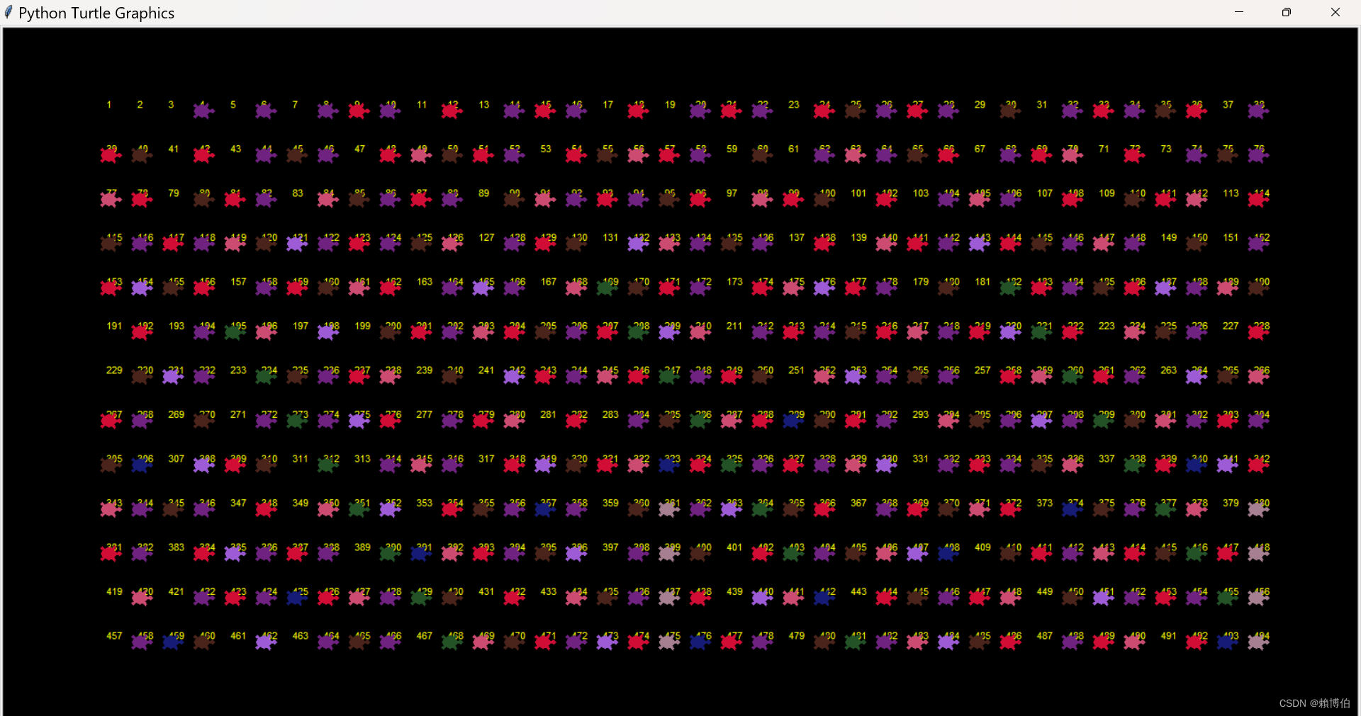
 以下我們分數個階段帶領讀者了解程式碼的設計
先測試用 turtle 在畫布上寫下數字 turtle.write()
此處用到 海龜在畫布寫字的指令 turtle.write()
# By Prof P-J Lai MATH NKNU 2016/4/8
# 測試在畫布上寫下數字
# draw 1,2,3,4,,,,on the canvas 在畫面依序寫出1,2,3,4,,,,50

from turtle import *
import random
import time

T=Turtle()
T.shape("turtle")
T.color("red")
#T.color("yellow")
T.turtlesize(2)
bgcolor(0,0,0)#RGB
T.pensize(5)
#T.pencolor("Green")

T.penup()
T.setpos(-650,0)
for i in range(1,51):
    #T.write(i,True)
    T.write(i) # 'Flase' means words will overlape the path
    T.fd(20)

T.setpos(-650,-50)
for i in range(51,80):
    T.write(i,True,font=('Arial', 15, 'italic'))
    T.fd(20)
Ex: 請同學練習, 在畫布上寫下整數 1 到 20, 1 到 10 排列在第一橫排, 11 到 20 排列在第二橫排, 大小與間隙自己調整, 使用何種字體, 與是否斜體、粗體等, 自己嘗試. 
在寫下的某個數字上, 令 turtle 在此數字蓋印, 代表刪去
# By Prof P-J Lai MATH NKNU 2016/4/8
# drawInteger_2_eraseByStamp_Lai.py
# 在寫下的某個數字上, 令 turtle 在此數字蓋印, 代表刪去.

from turtle import *
import random
import time

T=Turtle()
T.shape("turtle")
T.color("red")
#T.color("yellow")
T.turtlesize(2)
#bgcolor(0,0,0)#RGB
T.pensize(5)
#T.pencolor("Green")

T.penup()
T.setpos(-650,0)
for i in range(1,51):
    #T.write(i,True)
    T.write(i) # 'Flase' means words will overlape the path
    T.fd(20)

T.setpos(-650,-50)
for i in range(51,80):
    T.write(i,True,font=('Arial', 15, 'italic'))
    T.fd(20)

#reset 3 seconds
time.sleep(1)

# erase some integers 把一些數字擦除
T.shape('square')
T.turtlesize(2)
T.color('black')
T.setpos(-650,0)
for i in range(1,10):
    T.stamp()
    T.fd(20)
注意: turtle.write(arg, move=False, align='left', font=('Arial', 8, 'normal')) 預設是 align=’left’ move = False
如果 move = True 則海龜會讓出字的空間, 產生偏移, 如果要用 黑色蓋印把數字蓋住, 會出現沒法蓋對位置的情況, 因為 數字與海龜原有的位置會有偏移, 只能用大一點的印 但是數字一多,偏移量就會累積.
即使 move=False, 還是會偏移, 偏移量會小一些.
依據篩去法程式, 令 turtle 在篩去的數字蓋印, 代表刪去
以下是博主的程式碼, 並沒有系統化, 以下是N=500, 來設計跟呈現動畫面, (注意: 當 N 改變時, 例如 N=100, 版面配置(數字的大小與位置)就會不適合. 後面會請同學練習, 當N=50 時 , 如何修改程式碼, 讓版面數字的排放是適當的?)
# By Prof P-J Lai MATH NKNU 2016/4/8
# drawInteger_Eratosthenes_Lai.py
# draw 1,2,3,4,,,,on the canvas 在畫面依序寫出1,2,3,4,,,,50
# And let turtle jump and stamp to show Eratosthenes sieve
# T.write(i,True,font=('Arial', 15, 'italic'))

#此處可以改進成一般最快的寫法:
#for j in range(i*i, m, i):
#               numbers[j] = False
#20220307

from turtle import *
from random import *
import math

T=Turtle()
T.shape("turtle")
#T.color("red")
T.color("yellow")
T.turtlesize(1)
bgcolor(0,0,0)#RGB
T.pensize(5)
#T.pencolor("Green")
#T.speed(0)
T.speed(0)
#tracer(2,10)
T.ht()

#####################################
# print number 1 ~ 494
T.penup()
T.setpos(-650,300)
for i in range(1,39):
    T.write(i)
    T.fd(35)

T.setpos(-650,250)
for i in range(39,39+38):
    T.write(i)
    T.fd(35)

T.setpos(-650,200)
for i in range(39+38,39+2*38):
    T.write(i)
    T.fd(35)

T.setpos(-650,150)
for i in range(39+2*38,39+3*38):
    T.write(i)
    T.fd(35)

T.setpos(-650,100)
for i in range(39+3*38,39+4*38):
    T.write(i)
    T.fd(35)

T.setpos(-650,50)
for i in range(39+4*38,39+5*38):
    T.write(i)
    T.fd(35)

T.setpos(-650,0)
for i in range(39+5*38,39+6*38):
    T.write(i)
    T.fd(35)

T.setpos(-650,-50)
for i in range(39+6*38,39+7*38):
    T.write(i)
    T.fd(35)

T.setpos(-650,-100)
for i in range(39+7*38,39+8*38):
    T.write(i)
    T.fd(35)

T.setpos(-650,-150)
for i in range(39+8*38,39+9*38):
    T.write(i)
    T.fd(35)

T.setpos(-650,-200)
for i in range(39+9*38,39+10*38):
    T.write(i)
    T.fd(35)

T.setpos(-650,-250)
for i in range(39+10*38,39+11*38):
    T.write(i)
    T.fd(35)

T.setpos(-650,-300)
for i in range(39+11*38,39+12*38):
    T.write(i)
    T.fd(35)

############################################

def coord(n):
    row=(n-1)//38
    column=(n-1)%38
    return(-650+column*35,300-row*50)


#Sieve of Eratosthenes
#此處可以改進成一般最快的寫法:
#for j in range(i*i, m, i):
##                numbers[j] = False
#20220307


N=494
Limit=math.ceil(math.sqrt(N))
Prime=[]
primeList=[]

for i in range(0,N+1):
    Prime.append(1)

# Prime=[ 1 for x in range(1,N+1)]

T.speed(6)
for i in range(2,Limit+1):
    if Prime[i]==1:
        T.color(random(),random(),random())
        for j in range(i*i,N+1):
            if j%i==0:
                T.setpos(coord(j))
                T.stamp()
                Prime[j]=0

for i in range(2,N+1):
    if Prime[i]==1:
        primeList.append(i)

print(primeList)
輸出的畫面:
>>>
= RESTART: D:\NEW_筆電的\網路免費軟體資料\Python教學\Python數論\turtle跑Eratosthenes\drawInteger_Eratosthenes_Lai.py
[2, 3, 5, 7, 11, 13, 17, 19, 23, 29, 31, 37, 41, 43, 47, 53, 59, 61, 67, 71, 73, 79, 83, 89, 97, 101, 103, 107, 109, 113, 127, 131, 137, 139, 149, 151, 157, 163, 167, 173, 179, 181, 191, 193, 197, 199, 211, 223, 227, 229, 233, 239, 241, 251, 257, 263, 269, 271, 277, 281, 283, 293, 307, 311, 313, 317, 331, 337, 347, 349, 353, 359, 367, 373, 379, 383, 389, 397, 401, 409, 419, 421, 431, 433, 439, 443, 449, 457, 461, 463, 467, 479, 487, 491]
 Ex1: 當 N 改變時, 例如 N=100, 原程式碼呈現的版面配置(數字的大小與位置)就會不適合. 後面會請同學練習, 當N=50 時 , 如何修改程式碼, 讓版面數字的排放是適當的?
Ex2: 改進成, 當 N 改變時, 例如 N=100, 版面配置(數字的大小位置)會自動調整.
Ex: 此處可以改進成一般網路上效能最快的寫法(例如SciPy官網篩去法例子的寫法) (revised 20220307): ==迴圈增加一個 間格 i 的跳躍!==
for j in range(i*i, m, i):
    numbers[j] = False
Ex2: 改進成, 當 N 改變時, 例如 N=100, 版面配置(數字的大小位置)會自動調整.
2.6 Fermat primlity test 費馬質數檢測
理論介紹可以參考:
- 李永樂老師, 如何快速篩選質數?費馬素性檢驗和米勒-拉賓測試, https://youtu.be/E5vtn_OIe-c link
- 王碩, 董文馨, 張舒行, 張ㄗㄜˊ, 李秉倫, Python 算法設計與分析, 14.3.1.
- Fermat primality test, Wiki, https://en.wikipedia.org/wiki/Fermat_primality_test link.
- Carmichael number, Wiki, https://en.wikipedia.org/wiki/Carmichael_number link
以下常稱為費馬小定理:
Theorem 5.1 Fermat’s theorem Let $p$ be a prime and suppose that $p \nmid a$. Then $a^{p-1} \equiv 1 \; (mod \; p)$.
費馬質數檢測 則是利用 費馬小定理的反向敘述, 反向敘述不一定成立,
反向敘述 發生的狀況可以分兩種:
- n 是合成數(例如 n=341=11*31), 可以找到 a 使得 $a^{341-1} \equiv 1 \; (mod \; 341)$, 例如 a=2, 4, 8 等等, 此時我們稱 n=341 是關於 2 的費馬偽質數, 或 341 是關於 8 的費馬偽質數, 等等. (Ref: 王碩, 董文馨, 張舒行, 張ㄗㄜˊ, 李秉倫, Python 算法設計與分析, 人民郵電, 2020.)
- 存在一種數, 叫 Carmichael number 卡米歇爾數, 定義 n 為一個卡米歇爾數, 如果使得 所有與 n 互質的數 a, 都有 $a^{n-1} \equiv 1 \; (mod \; n)$, 例如 n= 561, 1105 等等, 都符合 卡米歇爾數的定義.
以下我們用 列表解析式 list comprehension 的語法, 輕鬆檢驗 341 的狀況, 發現會讓 341 通過檢驗的 a 很多, 例如 a=2, 4, 8 等等, 即使存在很多這樣的 2, 4, 8 等等的使得 $2^{341-1} \equiv 1 \; (mod \; 341)$, 還是無法理論上保證, 341是質數, 如果早已知道341是合成數, 就稱此種 a 稱為 Fermat liar費馬騙子數. 如果是使得 $a^{341-1} \not\equiv 1 \; (mod \; 341)$, 此種 a 稱為 Fermat witness費馬證人數, 例如 a=3, 6, 9 等等, 這樣的 Fermat witness 費馬證人數, ==只要找到一個, 就可以使我們立刻斷定 341 是合成數!== ($\because (P \Rightarrow Q) \; \equiv \; (\sim Q \Rightarrow \sim P)$).
註: 列表解析式 list comprehension 也有 iterator 的語法, 就是把中括號改成小括號即可. 例如把 [a**340 % 341 for a in range(2,341)] 改成 (a**340 % 341 for a in range(2,341)])
列表解析式觀察費馬偽質數
列表解析式 list comprehension 的語法: [a**340 % 341 for a in range(2,341)] 以下我們發現有的 算出來是 1, 有的不是, 但是必須是與341互質的數算出的不是1, 我們才能斷定 341是合成數, 底下列出的結果, 由於只有部分是與 341 互質, 所以難以一目瞭然,
>>> 31*11
341
>>>[ i**340 % 341 for i in range(2,341)]
[1, 56, 1, 67, 56, 56, 1, 67, 67, 253, 56, 67, 56, 1, 1, 56, 67, 56, 67, 67,
 253, 1, 56, 56, 67, 1, 56, 1, 1, 155, 1, 187, 56, 1, 67, 56, 56, 1, 67, 67,
 67, 56, 253, 56, 1, 1, 56, 67, 56, 67, 67, 67, 1, 242, 56, 67, 1, 56, 1,
 1, 155, 1, 1, 56, 187, 67, 56, 56, 1, 67, 67, 67, 56, 67, 56, 187, 1, 56,
 67, 56, 67, 67, 67, 1, 56, 56, 253, 1, 56, 1, 1, 155, 1, 1, 56, 1, 67,
 242, 56, 1, 67, 67, 67, 56, 67, 56, 1, 1, 242, 67, 56, 67, 67, 67, 1,
 56, 56, 67, 1, 242, 1, 1, 155, 1, 1, 56, 1, 67, 56, 56, 187, 67, 67,
67, 56, 67, 56, 1, 1, 56, 67, 242, 67, 67, 67, 1, 56, 56, 67, 1, 56, 1, 187, 155, 1, 1, 56, 1, 67, 56, 56, 1, 67, 253, 67, 56, 67, 56, 1, 1, 56,
67, 56, 67, 253, 67, 1, 56, 56, 67, 1, 56, 1, 1, 155, 187, 1, 56, 1,
67, 56, 56, 1, 67, 67, 67, 242, 67, 56, 1, 1, 56, 67, 56, 67, 67,
67, 187, 56, 56, 67, 1, 56, 1, 1, 155, 1, 1, 242, 1, 67, 56, 56,
1, 67, 67, 67, 56, 67, 242, 1, 1, 56, 67, 56, 67, 67, 67, 1, 56,
  242, 67, 1, 56, 1, 1, 155, 1, 1, 56, 1, 253, 56, 56, 1, 67, 67, 67, 56, 67, 56, 1, 187, 56, 67, 56, 67, 67, 67, 1, 56, 56, 67, 187, 56, 1,
 1, 155, 1, 1, 56, 1, 67, 56, 242, 1, 67, 67, 67, 56, 67, 56, 1, 1, 56, 253, 56, 67, 67, 67, 1, 56, 56, 67, 1, 56, 187, 1, 155, 1, 1, 56, 1,
 67, 56, 56, 1, 253, 67, 67, 56, 67, 56, 1, 1, 56, 67, 56, 253,
  67, 67, 1, 56, 56, 67, 1, 56, 1, 1]
Ex: 因為只需檢驗與 n=341 互質的 a, 請使用 math.gcd(), 結合 列表解析式 list comprehension 的 if 語法: 將不互質的 a 去掉, 再看結果, 是否更清楚. Ans:
[a**340 % 341 for a in range(2,341) if math.gcd(a,341)==1]
將不互質的 a 去掉, 則結果相當清楚, 一目了然, 仍然出現很多不是 1 的結果, 顯示 341 是合成數.
import math
[ i**340 % 341 for i in range(2,341) if math.gcd(i,341)==1]
[1, 56, 1, 67, 56, 56, 1, 67, 67, 56, 67, 56, 1, 1, 56, 67, 56, 67, 67, 1,
 56, 56, 67, 1, 56, 1, 1, 1, 56, 1, 67, 56, 56, 1, 67, 67, 67, 56, 56, 1, 1,
56, 67, 56, 67, 67, 67, 1, 56, 67, 1, 56, 1, 1, 1, 1, 56, 67, 56, 56,
1, 67, 67, 67, 56, 67, 56, 1, 56, 67, 56, 67, 67, 67, 1, 56, 56, 1, 56, 1, 1, 1, 1, 56, 1, 67, 56, 1, 67, 67, 67, 56, 67, 56, 1, 1, 67, 56, 67, 67, 67,
 1, 56, 56, 67, 1, 1, 1, 1, 1, 56, 1, 67, 56, 56, 67, 67, 67, 56, 67, 56, 1, 1, 56, 67, 67, 67, 67, 1, 56, 56, 67, 1, 56, 1, 1, 1, 56, 1, 67, 56, 56, 1, 67, 67, 56, 67, 56, 1, 1, 56, 67, 56, 67, 67, 1, 56, 56, 67, 1, 56, 1, 1, 1, 56, 1, 67, 56, 56, 1, 67, 67, 67, 67, 56, 1, 1, 56, 67, 56, 67, 67, 67, 56, 56, 67, 1, 56, 1, 1, 1, 1, 1, 67, 56, 56, 1, 67, 67, 67, 56, 67, 1, 1, 56, 67, 56, 67, 67, 67, 1, 56, 67, 1, 56, 1, 1, 1, 1, 56, 1, 56, 56, 1, 67, 67, 67, 56, 67, 56, 1, 56, 67, 56, 67, 67, 67, 1, 56, 56, 67, 56, 1, 1, 1, 1, 56, 1, 67, 56, 1, 67, 67, 67, 56, 67, 56, 1, 1, 56, 56, 67, 67, 67, 1, 56, 56, 67, 1, 56, 1, 1, 1, 56, 1, 67, 56, 56, 1, 67, 67, 56, 67, 56, 1, 1, 56, 67, 56, 67, 67, 1, 56, 56, 67, 1, 56, 1, 1]
Ex: 用 numpy.where() 的指令, 抓出 使得 $a^{341-1} \equiv 1 \; (mod \; 341)$ 成立的所有 a (小於 341). Ans:
小心 , 由於 NumPy 類似 C 或是 Matlab 的科學計算, 整數太大與會溢位, 不像==原生的 Python 可以任意長整數==, 所以最好先用 原生的 Python 計算大的次方, 再轉成 numpy.array 的格式
>>> list341 = [ i**340 % 341 for i in range(2,341)]
>>> import numpy
>>> listNp341 = numpy.array(list341)
>>>> numpy.where(listNp341==1)
(array([  0,   2,   6,  13,  14,  21,  25,  27,  28,  30,  33,  37,  44,
        45,  52,  56,  58,  59,  61,  62,  68,  76,  83,  87,  89,  90,
        92,  93,  95,  99, 106, 107, 114, 118, 120, 121, 123, 124, 126,
       137, 138, 145, 149, 151, 154, 155, 157, 161, 168, 169, 176, 180,
       182, 183, 186, 188, 192, 199, 200, 211, 213, 214, 216, 217, 219,
       223, 230, 231, 238, 242, 244, 245, 247, 248, 250, 254, 261, 269,
       275, 276, 278, 279, 281, 285, 292, 293, 300, 304, 307, 309, 310,
       312, 316, 323, 324, 331, 335, 337, 338], dtype=int64),)
>>>index341 = numpy.where(listNp341==1)
>>>index341
(array([  0,   2,   6,  13,  14,  21,  25,  27,  28,  30,  33,  37,  44,
        45,  52,  56,  58,  59,  61,  62,  68,  76,  83,  87,  89,  90,
        92,  93,  95,  99, 106, 107, 114, 118, 120, 121, 123, 124, 126,
       137, 138, 145, 149, 151, 154, 155, 157, 161, 168, 169, 176, 180,
       182, 183, 186, 188, 192, 199, 200, 211, 213, 214, 216, 217, 219,
       223, 230, 231, 238, 242, 244, 245, 247, 248, 250, 254, 261, 269,
       275, 276, 278, 279, 281, 285, 292, 293, 300, 304, 307, 309, 310,
       312, 316, 323, 324, 331, 335, 337, 338], dtype=int64),)
>>>index341[0]
array([  0,   2,   6,  13,  14,  21,  25,  27,  28,  30,  33,  37,  44,
        45,  52,  56,  58,  59,  61,  62,  68,  76,  83,  87,  89,  90,
        92,  93,  95,  99, 106, 107, 114, 118, 120, 121, 123, 124, 126,
       137, 138, 145, 149, 151, 154, 155, 157, 161, 168, 169, 176, 180,
       182, 183, 186, 188, 192, 199, 200, 211, 213, 214, 216, 217, 219,
       223, 230, 231, 238, 242, 244, 245, 247, 248, 250, 254, 261, 269,
       275, 276, 278, 279, 281, 285, 292, 293, 300, 304, 307, 309, 310,
       312, 316, 323, 324, 331, 335, 337, 338], dtype=int64)
>>>len(index341[0])
99
>>> index341+ numpy.ones((1, len(index341)))*2
array([[  2.,   4.,   8.,  15.,  16.,  23.,  27.,  29.,  30.,  32.,  35.,
         39.,  46.,  47.,  54.,  58.,  60.,  61.,  63.,  64.,  70.,  78.,
         85.,  89.,  91.,  92.,  94.,  95.,  97., 101., 108., 109., 116.,
        120., 122., 123., 125., 126., 128., 139., 140., 147., 151., 153.,
        156., 157., 159., 163., 170., 171., 178., 182., 184., 185., 188.,
        190., 194., 201., 202., 213., 215., 216., 218., 219., 221., 225.,
        232., 233., 240., 244., 246., 247., 249., 250., 252., 256., 263.,
        271., 277., 278., 280., 281., 283., 287., 294., 295., 302., 306.,
        309., 311., 312., 314., 318., 325., 326., 333., 337., 339., 340.]])
# 以下寫法會出錯, 因為有廣播功能, 所以結果還是對,  但是容易混淆
index341+ numpy.ones((1, len(index341)))*2
array([[  2.,   4.,   8.,  15.,  16.,  23.,  27.,  29.,  30.,  32.,  35.,
         39.,  46.,  47.,  54.,  58.,  60.,  61.,  63.,  64.,  70.,  78.,
         85.,  89.,  91.,  92.,  94.,  95.,  97., 101., 108., 109., 116.,
        120., 122., 123., 125., 126., 128., 139., 140., 147., 151., 153.,
        156., 157., 159., 163., 170., 171., 178., 182., 184., 185., 188.,
        190., 194., 201., 202., 213., 215., 216., 218., 219., 221., 225.,
        232., 233., 240., 244., 246., 247., 249., 250., 252., 256., 263.,
        271., 277., 278., 280., 281., 283., 287., 294., 295., 302., 306.,
        309., 311., 312., 314., 318., 325., 326., 333., 337., 339., 340.]])
# 以下才是較穩健的寫法:
>>>index341[0]+ numpy.ones((1, len(index341[0])))*2
array([[  2.,   4.,   8.,  15.,  16.,  23.,  27.,  29.,  30.,  32.,  35.,
         39.,  46.,  47.,  54.,  58.,  60.,  61.,  63.,  64.,  70.,  78.,
         85.,  89.,  91.,  92.,  94.,  95.,  97., 101., 108., 109., 116.,
        120., 122., 123., 125., 126., 128., 139., 140., 147., 151., 153.,
        156., 157., 159., 163., 170., 171., 178., 182., 184., 185., 188.,
        190., 194., 201., 202., 213., 215., 216., 218., 219., 221., 225.,
        232., 233., 240., 244., 246., 247., 249., 250., 252., 256., 263.,
        271., 277., 278., 280., 281., 283., 287., 294., 295., 302., 306.,
        309., 311., 312., 314., 318., 325., 326., 333., 337., 339., 340.]])

>>>numpy.ones((1, len(index341)))*2
array([[2.]])
>>>numpy.ones((1, len(index341[0])))*2
array([[2., 2., 2., 2., 2., 2., 2., 2., 2., 2., 2., 2., 2., 2., 2., 2.,
        2., 2., 2., 2., 2., 2., 2., 2., 2., 2., 2., 2., 2., 2., 2., 2.,
        2., 2., 2., 2., 2., 2., 2., 2., 2., 2., 2., 2., 2., 2., 2., 2.,
        2., 2., 2., 2., 2., 2., 2., 2., 2., 2., 2., 2., 2., 2., 2., 2.,
        2., 2., 2., 2., 2., 2., 2., 2., 2., 2., 2., 2., 2., 2., 2., 2.,
        2., 2., 2., 2., 2., 2., 2., 2., 2., 2., 2., 2., 2., 2., 2., 2.,
        2., 2., 2.]])
以上列出的 2,4,8,15,16,,就是使得 $a^{341-1} \equiv 1 \; (mod \; 341)$ 的 a. 以上是屬於第1種的情形, 就是合成數 341, 會同時有 費馬騙子數, 與費馬證人數.
第2種情形, 稱為 Carmichael number 卡米歇爾數, 則是所有與 n 互質的數 a, 都是費馬證人數! 此種 Carmichael number 卡米歇爾數, 儘管數量很稀少, 還是使得費馬質數檢測的使用不如米勒拉賓質數檢測等其他機率型的質數檢測演算法, 但是 OpenPFGW, PGP 是使用費馬質數檢測.
最小的 卡米歇爾數 為 $561=3\times 11 \times 7$,
接下來的 6 個卡米歇爾數 (sequence A002997 in the OEIS):
| 1105 = 5×13×17 (4 | 1104, 12 | 1104, 16 | 1104) |
| 1729 = 7×13×19 (6 | 1728, 12 | 1728, 18 | 1728) |
| 2465 = 5×17×29 (4 | 2464, 16 | 2464, 28 | 2464) |
| 2821 = 7×13×31 (6 | 2820, 12 | 2820, 30 | 2820) |
| 6601 = 7×23×41 (6 | 6600, 22 | 6600, 40 | 6600) |
| 8911 = 7×19×67 (6 | 8910, 18 | 8910, 66 | 8910) |
>>> [a**560 % 561  for a in range(2,561)]
[1, 375, 1, 1, 375, 1, 1, 375, 1, 154, 375, 1, 1, 375, 1, 34,
375, 1, 1, 375, 154, 1, 375, 1, 1, 375, 1, 1, 375, 1, 1, 528,
 34, 1, 375, 1, 1, 375, 1, 1, 375, 1, 154, 375, 1, 1, 375, 1,
 1, 408, 1, 1, 375, 154, 1, 375, 1, 1, 375, 1, 1, 375, 1, 1,
 528, 1, 34, 375, 1, 1, 375, 1, 1, 375, 1, 154, 375, 1, 1, 375, 1, 1, 375, 34, 1, 375, 154, 1, 375, 1, 1, 375, 1, 1, 375, 1, 1, 528, 1, 1, 408, 1, 1, 375, 1, 1, 375, 1, 154, 375, 1, 1, 375, 1, 1, 375, 1, 34, 375, 154, 1, 375, 1, 1, 375, 1, 1, 375, 1, 1, 528, 1, 1, 375, 34, 1, 375, 1, 1, 375, 1, 154, 375, 1, 1, 375, 1, 1, 375, 1, 1, 408, 154, 1, 375, 1, 1, 375, 1, 1, 375, 1, 1, 528, 1, 1, 375, 1, 34, 375, 1, 1, 375, 1, 154, 375, 1, 1, 375, 1, 1, 375, 1, 1, 375, 187, 1, 375, 1, 1, 375, 1, 1, 375, 1, 1, 528, 1, 1, 375, 1, 1, 408, 1, 1, 375, 1, 154, 375, 1, 1, 375, 1, 1, 375, 1, 1, 375, 154, 34, 375, 1, 1, 375, 1, 1, 375, 1, 1, 528, 1, 1, 375, 1, 1, 375, 34, 1, 375, 1, 154, 375, 1, 1, 375, 1, 1, 375, 1, 1, 375, 154, 1, 408, 1, 1, 375, 1, 1, 375, 1, 1, 528, 1, 1, 375, 1, 1, 375, 1, 34, 375, 1, 154, 375, 1, 1, 375, 1, 1, 375, 1, 1, 375, 154, 1, 375, 34, 1, 375, 1, 1, 375, 1, 1, 528, 1, 1, 375, 1, 1, 375, 1, 1, 408, 1, 154, 375, 1, 1, 375, 1, 1, 375, 1, 1, 375, 154, 1, 375, 1, 34, 375, 1, 1, 375, 1, 1, 528, 1, 1, 375, 1, 1, 375, 1, 1, 375, 34, 154, 375, 1, 1, 375, 1, 1, 375, 1, 1, 375, 154, 1, 375, 1, 1, 408, 1, 1, 375, 1, 1, 528, 1, 1, 375, 1, 1, 375, 1, 1, 375, 1, 187, 375, 1, 1, 375, 1, 1, 375, 1, 1, 375, 154, 1, 375, 1, 1, 375, 34, 1, 375, 1, 1, 528, 1, 1, 375, 1, 1, 375, 1, 1, 375, 1, 154, 408, 1, 1, 375, 1, 1, 375, 1, 1, 375, 154, 1, 375, 1, 1, 375, 1, 34, 375, 1, 1, 528, 1, 1, 375, 1, 1, 375, 1, 1, 375, 1, 154, 375, 34, 1, 375, 1, 1, 375, 1, 1, 375, 154, 1, 375, 1, 1, 375, 1, 1, 408, 1, 1, 528, 1, 1, 375, 1, 1, 375, 1, 1, 375, 1, 154, 375, 1, 34, 375, 1, 1, 375, 1, 1, 375, 154, 1, 375, 1, 1, 375, 1, 1, 375, 34, 1, 528, 1, 1, 375, 1, 1, 375, 1, 1, 375, 1, 154, 375, 1, 1, 408, 1, 1, 375, 1, 1, 375, 154, 1, 375, 1, 1, 375, 1, 1, 375, 1, 34, 528, 1, 1, 375, 1, 1, 375, 1, 1, 375, 1, 154, 375, 1, 1, 375, 34, 1, 375, 1, 1, 375, 154, 1, 375, 1, 1, 375, 1, 1, 375, 1, 1]
Ex: 檢驗以上 Wiki 列出的數 561, 1105 等符合 卡米歇爾數的定義. (參考: 王碩, 董文馨, 張舒行, 張ㄗㄜˊ, 李秉倫, Python 算法設計與分析, 14.3.1, P.231, 指出, ==比 $2.5 \times 10^{10}$ 小的 卡米歇爾數只有 2163 個==.)
以下檢驗 561 的計算狀況 列表解析式 list comprehension 的語法: [a**560 % 561 for a in range(2,561)] 底下列出的結果, 由於只有部分是與 561 互質, 所以難以一目瞭然,
>>> [a**560 % 561  for a in range(2,561)]
[1, 375, 1, 1, 375, 1, 1, 375, 1, 154, 375, 1, 1, 375, 1, 34,
 375, 1, 1, 375, 154, 1, 375, 1, 1, 375, 1, 1, 375, 1, 1, 528,
  34, 1, 375, 1, 1, 375, 1, 1, 375, 1, 154, 375, 1, 1, 375, 1,
   1, 408, 1, 1, 375, 154, 1, 375, 1, 1, 375, 1, 1, 375, 1, 1,
    528, 1, 34, 375, 1, 1, 375, 1, 1, 375, 1, 154, 375, 1, 1, 375, 1, 1, 375, 34, 1, 375, 154, 1, 375, 1, 1, 375, 1, 1, 375, 1, 1, 528, 1, 1, 408, 1, 1, 375, 1, 1, 375, 1, 154, 375, 1, 1, 375, 1, 1, 375, 1, 34, 375, 154, 1, 375, 1, 1, 375, 1, 1, 375, 1, 1, 528, 1, 1, 375, 34, 1, 375, 1, 1, 375, 1, 154, 375, 1, 1, 375, 1, 1, 375, 1, 1, 408, 154, 1, 375, 1, 1, 375, 1, 1, 375, 1, 1, 528, 1, 1, 375, 1, 34, 375, 1, 1, 375, 1, 154, 375, 1, 1, 375, 1, 1, 375, 1, 1, 375, 187, 1, 375, 1, 1, 375, 1, 1, 375, 1, 1, 528, 1, 1, 375, 1, 1, 408, 1, 1, 375, 1, 154, 375, 1, 1, 375, 1, 1, 375, 1, 1, 375, 154, 34, 375, 1, 1, 375, 1, 1, 375, 1, 1, 528, 1, 1, 375, 1, 1, 375, 34, 1, 375, 1, 154, 375, 1, 1, 375, 1, 1, 375, 1, 1, 375, 154, 1, 408, 1, 1, 375, 1, 1, 375, 1, 1, 528, 1, 1, 375, 1, 1, 375, 1, 34, 375, 1, 154, 375, 1, 1, 375, 1, 1, 375, 1, 1, 375, 154, 1, 375, 34, 1, 375, 1, 1, 375, 1, 1, 528, 1, 1, 375, 1, 1, 375, 1, 1, 408, 1, 154, 375, 1, 1, 375, 1, 1, 375, 1, 1, 375, 154, 1, 375, 1, 34, 375, 1, 1, 375, 1, 1, 528, 1, 1, 375, 1, 1, 375, 1, 1, 375, 34, 154, 375, 1, 1, 375, 1, 1, 375, 1, 1, 375, 154, 1, 375, 1, 1, 408, 1, 1, 375, 1, 1, 528, 1, 1, 375, 1, 1, 375, 1, 1, 375, 1, 187, 375, 1, 1, 375, 1, 1, 375, 1, 1, 375, 154, 1, 375, 1, 1, 375, 34, 1, 375, 1, 1, 528, 1, 1, 375, 1, 1, 375, 1, 1, 375, 1, 154, 408, 1, 1, 375, 1, 1, 375, 1, 1, 375, 154, 1, 375, 1, 1, 375, 1, 34, 375, 1, 1, 528, 1, 1, 375, 1, 1, 375, 1, 1, 375, 1, 154, 375, 34, 1, 375, 1, 1, 375, 1, 1, 375, 154, 1, 375, 1, 1, 375, 1, 1, 408, 1, 1, 528, 1, 1, 375, 1, 1, 375, 1, 1, 375, 1, 154, 375, 1, 34, 375, 1, 1, 375, 1, 1, 375, 154, 1, 375, 1, 1, 375, 1, 1, 375, 34, 1, 528, 1, 1, 375, 1, 1, 375, 1, 1, 375, 1, 154, 375, 1, 1, 408, 1, 1, 375, 1, 1, 375, 154, 1, 375, 1, 1, 375, 1, 1, 375, 1, 34, 528, 1, 1, 375, 1, 1, 375, 1, 1, 375, 1, 154, 375, 1, 1, 375, 34, 1, 375, 1, 1, 375, 154, 1, 375, 1, 1, 375, 1, 1, 375, 1, 1]
因為只需檢驗與 n=561 互質的 a, 我們使用 math.gcd(), 結合 列表解析式 list comprehension 的 if 語法:
[a**560 % 561 for a in range(2,561) if math.gcd(a,561)==1]
將不互質的 a 去掉, 則結果相當清楚, 一目了然!
>>> import math
>>> [a**560 % 561  for a in range(2,561) if math.gcd(a,561)==1]
[1, 1, 1, 1, 1, 1, 1, 1, 1, 1, 1, 1, 1, 1, 1, 1, 1, 1, 1, 1, 1,
1, 1, 1, 1, 1, 1, 1, 1, 1, 1, 1, 1, 1, 1, 1, 1, 1, 1, 1, 1, 1,
1, 1, 1, 1, 1, 1, 1, 1, 1, 1, 1, 1, 1, 1, 1, 1, 1, 1, 1, 1, 1,
1, 1, 1, 1, 1, 1, 1, 1, 1, 1, 1, 1, 1, 1, 1, 1, 1, 1, 1, 1, 1,
1, 1, 1, 1, 1, 1, 1, 1, 1, 1, 1, 1, 1, 1, 1, 1, 1, 1, 1, 1, 1,
1, 1, 1, 1, 1, 1, 1, 1, 1, 1, 1, 1, 1, 1, 1, 1, 1, 1, 1, 1, 1, 1, 1, 1, 1, 1, 1, 1, 1, 1, 1, 1, 1, 1, 1, 1, 1, 1, 1, 1, 1, 1, 1, 1, 1, 1, 1, 1, 1, 1, 1, 1, 1, 1, 1, 1, 1, 1, 1, 1, 1, 1, 1, 1, 1, 1, 1, 1, 1, 1, 1, 1, 1, 1, 1, 1, 1, 1, 1, 1, 1, 1, 1, 1, 1, 1, 1, 1, 1, 1, 1, 1, 1, 1, 1, 1, 1, 1, 1, 1, 1, 1, 1, 1, 1, 1, 1, 1, 1, 1, 1, 1, 1, 1, 1, 1, 1, 1, 1, 1, 1, 1, 1, 1, 1, 1, 1, 1, 1, 1, 1, 1, 1, 1, 1, 1, 1, 1, 1, 1, 1, 1, 1, 1, 1, 1, 1, 1, 1, 1, 1, 1, 1, 1, 1, 1, 1, 1, 1, 1, 1, 1, 1, 1, 1, 1, 1, 1, 1, 1, 1, 1, 1, 1, 1, 1, 1, 1, 1, 1, 1, 1, 1, 1, 1, 1, 1, 1, 1, 1, 1, 1, 1, 1, 1, 1, 1, 1, 1, 1, 1, 1, 1, 1, 1, 1, 1, 1, 1, 1, 1, 1, 1, 1]
發現, 所有與 n=561 互質的數 a, 確實都會 $a^{n-1} \equiv 1 \; (mod \; n)$! 所以 n=561 確實是 米歇爾數.
Ex: 用 Python 找出 不在以上 Wiki 列出的 卡米歇爾數.
費馬質數檢測的 flowchart
利用 費馬小定理的反向敘述來檢測質數, 就是, 假設你想檢測 n 是否為質數, 則隨機挑幾個與 n 互質的數 a, 看 $a^{n-1} \equiv 1 \; (\mod \; n)$ 是否成立, 如果有遇到一個 a 使得 $a^{n-1} \not\equiv 1 \; (\mod \; n)$, 則可以立刻得到 $n$ 不是質數, 如果嘗試夠多個 a, 都得到 $a^{n-1} \equiv 1 \; (\mod \; n)$, 此時只能說 n 是質數的可能性極大.
例如 341, 有 費馬騙子數 2,4,8,15,16, 使得 $a^{341-1} \equiv 1 \; (\mod \; 341)$ 成立. 另外也有費馬證人數 Fermat witness, 例如 a=3, 6, 9 等等, 使得 $a^{341-1} \not\equiv 1 \; (\mod \; 341)$ 成立, 這樣的數, 可以使我們立刻斷定 341 是合成數, 此種數, 數量也很多.
根據 王碩, 董文馨, 張舒行, 張ㄗㄜˊ, 李秉倫, Python 算法設計與分析, 14.3.1, P.231, 指出, ==隨機選出 a, “n 不是以 a 為底的偽質數” 的機率至少是 $50\%$==, 故 , 如果只做一次檢驗, 成功的機率至少是 $50\%$, 做兩次檢驗, 成功的機率至少是 $75\%$, ==如果做10次檢驗, 成功的機率至少是 $99.9\%$==.
# Fermat primality test
# By Prof. P-J Lai MATH NKNU 20250302
##>>> help('random.randint')
##Help on method randint in random:
##
##random.randint = randint(a, b) method of random.Random instance
##    Return random integer in range [a, b], including both end points.

# a**(n-1)%n
# 等價於 pow(a, n-1, n)

##The algorithm can be written as follows:
##
##Inputs: n: a value to test for primality, n>3; k: a parameter that determines the number of times to test for primality
##Output: composite if n is composite, otherwise probably prime
##Repeat k times:
##Pick a randomly in the range [2, n − 2]
##If {\displaystyle a^{n-1}\not \equiv 1{\pmod {n}}}a^\not \equiv 1{\pmod  n}, then return composite
##If composite is never returned: return probably prime
##The a values 1 and n-1 are not used as the equality holds for all n and all odd n respectively, hence testing them adds no value.


import random

def FermatPrimalityTest(n,k):

    times = k
    while times >= 1:
        a = random.randint(2,n-2)
        if a**(n-1)%n != 1:
        # 等價於 pow(a, n-1, n)
            return False

        times = times - 1

    return True

##輸出
##>>>
##============= RESTART: C:/Users/user/Desktop/FermatPrimalityTest.py ============

##>>> FermatPrimalityTest(101,3)
##True
##>>> FermatPrimalityTest(195,3)
##False
##>>> FermatPrimalityTest(421,3)
##True
##>>> FermatPrimalityTest(91,3)
##False
##>>> FermatPrimalityTest(91,3)
##False
##>>> FermatPrimalityTest(91,3)
##False
Ex: 寫一個 Python 程式搜尋例如 十萬100000或百萬1000000以內的所有卡米歇爾數.
2.7 Miller-Rabin test 米勒拉賓質數檢測
理論介紹可以參考:
以下主要參考 Wiki 的說明:
Lemma1: If p is prime, then the root of $X^2 \equiv 1 \mod n$ should be either $X \equiv 1 \mod n$ or $X \equiv -1 \mod n$. Pf: 請參考 Wiki.
由 Lemma1 可以得到
Lemma2: If n is prime, then for any $a \in {2,3,4,,,,n-1}$, we have that either $a^{d} \equiv 1 \mod n$ for some odd number $d >0.—–(1)$
or $a^{2^rd} \equiv -1 \mod n$ for some $r \ge 0.———(2)$
Pf: 假設 n 為質數 取 $a \in {2,3,4,,,,n-1}$ 此時由 費馬小定理, 有 $a^{n-1} \equiv 1 \mod n$ n 為質數, 如果 n=2, 則 (1) 一定成立, 如果 n>2, 則為奇數, 則有 n-1 為偶數, 可以表為 $n-1=2^sd$ 則 $a^{n-1} \equiv 1 \mod n$ 就可以寫成 $a^{2^sd} \equiv 1 \mod n$ 用冪次律整理, 抽出 2 次方: $(a^{d})^{2^s} \equiv 1 \mod n$, $((a^{d})^{2^{s-1}2} \equiv 1 \mod n$, $((a^{d})^{2^{s-1}})^2 \equiv 1 \mod n$. 根據前面的小引理Lemma1, 得到平方根只可能是 $\pm 1$, 也就是 $(a^{d})^{2^{s-1}}\equiv 1 \mod n$ or $(a^{d})^{2^{s-1}}\equiv -1 \mod n$
或者 更清楚一點表達 Let $X := (a^{d})^{2^{s-1}}$ 則有 $X^2 \equiv 1 \mod n$ 根據前面的 Lemma1, 得到 $X \equiv 1 \mod n$ or $X \equiv -1 \mod n$, 也就是 平方根 X 只可能是 $\pm 1$,
case1 : 假設我們得到的是 $X \equiv 1 \mod n$ 如果 $s>1$, 則 $X := (a^{d})^{2^{s-1}}$ 就可以再用冪次律整理, 抽出 2 次方: $X=((a^{d})^{2^{s-2}})^2 \equiv 1 \mod n$
可以令 Let $X1= ((a^{d})^{2^{s-2}})$, 則有 $(X1)^2 \equiv 1 \mod n$ 則可以再用一次 Lemma1, 得到平方根 X1 只可能是 $\pm 1$,
所以, ==如果每次都 mod 等於 1, 則可以把 $2^s$ 抽光==, 最後剩下 $a^{d} \equiv 1 \mod n$ 則得到 (1) 的狀況.
case2 : 假設我們得到的是 $X \equiv -1 \mod n$ 另一方面, 不管 $s=1$ 或 $s>1$, 如果是mod 等於 -1 的情況: $X \equiv -1 \mod n$. 則得到 (2) 的狀況: $a^{2^rd} \equiv -1 \mod n$ for some $r \ge 0$.
經過上面討論, 就知道一定會落入 (1) 或 (2) 的狀況.
得證.$\; \blacksquare$
根據 王碩, 董文馨, 張舒行, 張ㄗㄜˊ, 李秉倫, Python 算法設計與分析, 14.3.2, P.231, 指出, ==米勒拉賓質數檢測是在 費馬質數檢測的基礎上又添加了另外的判斷條件, 令 卡米歇爾數更難通過檢測!==
程式碼可以看:
- 王碩, 董文馨, 張舒行, 張ㄗㄜˊ, 李秉倫, Python 算法設計與分析, 14.3.3, P.233.
- 雲帝, Python Miller Rabin 米勒-拉宾素性检验, link
以下參考 王碩, 董文馨, 張舒行, 張ㄗㄜˊ, 李秉倫, Python 算法設計與分析, 14.3.3, P.233 的程式碼:
 # 以下參考 王碩, 董文馨, 張舒行, 張ㄗㄜˊ, 李秉倫, Python 算法設計與分析, 14.3.3, P.233 的程式碼
 # By Prof. P-J Lai MATH NKNU 20250403

from random import randrange

# 以 a 為底數, 檢查 n 是否為合數, n-1 = 2^k*d

def checkComposite(a,k,d,n):
    x = pow(a, d, n)
    if x == 1 or x == n-1:
        return False

    for _ in range(k-1):
        x = pow(x, 2, n)
        if x == n-1:
            return False

    return True

# n 是被檢驗的數, m 是精準度

# 判斷 n 是否不是合數

def miller_rabin(n, m):
    if n == 2 or n == 3:
        return True
    if n % 2 == 0:
        return False
    k = 0
    d = n-1
    # 計算 k  與 d
    while d % 2 ==0:
        k += 1
        d = d//2

    for _ in range(m):
        a = randrange(2, n-1)
        if checkComposite(a,k,d,n):
            return False
        return True
3. 用 sympy 求因數與質數
sympy 求因數的指令
sympy.factorint 列出因數與因數之次方(重數) sympy.primefactors 列出質因數
>>> import sympy
>>> sympy.primefactors(120)
[2, 3, 5]
>>> sympy.primefactors(17894)
[2, 23, 389]
>>> sympy.factorint(120)
{2: 3, 3: 1, 5: 1}
>>> sympy.factorint(17894)
{2: 1, 23: 1, 389: 1}
sympy才有與質數與密碼有關的指令
prevprime, nextprime, isprime, randprime, prime(), sieve(), primerange(a, b) primerange(a, b) 範圍包含 a, 不包含 b. prime(k) 產生第k個質數
>>> import sympy
>>> print([i for i in sympy.primerange(1,30)])
[2, 3, 5, 7, 11, 13, 17, 19, 23, 29]
>>> print([i for i in sympy.sieve.primerange(1,30)])
[2, 3, 5, 7, 11, 13, 17, 19, 23, 29]
P.310 The Sieve method, primerange, is generally faster but it will occupy more memory as the sieve stores values.
>>> sympy.isprime(100003)
True
>>> sympy.randprime(1,1000)
331

>>> sympy.factorint(100001)
{11: 1, 9091: 1}
4. primePy PyPI: Python 的其他質數模組
5. 測量以上各種不同求質數或質數檢測之寫法, 使用 time.time(), 比較它們的效能
Ex: 測量以上各種不同求質數或質數檢測之寫法, 使用 time.time(), 及 timeit.timeit 比較它們的效能
6. 展現 Python 呈現超長整數的能力: 孿生質數猜想: 用Python呈現 2009 為止最大的孿生質數 (Using Python to show the biggest twin prime pairs up to 2009)
Ex: 寫出 Python 程式, 列出給定範圍之所有孿生質數.
展現 Python 呈現超長整數的能力 Pyhton的整數位數在內存記憶允許之下, 真的整數幾乎無限制,
整數太長時, 在IDLE無法顯示,會卡住, 他會顯示建議你複製或用view, 用view還是當住, 我是按右鍵copy, 再貼入純文字檔, 就可以了
應數一整數論: Burton 課本 sec3.3 The Goldbach conjecture P. 50 20200515 用Python算2009發現最大之孿生質數, 孿生質數猜想 孿生質數就是相隔2的兩個質數, 2009年發現最大的是 65516468355*pow(2,333333)-1 65516468355*pow(2,333333)+1 是否存在無限多組, 目前還未證明出, 但是電腦搜尋似乎是正確的猜想 證明Pyhton的整數位數在內存記憶允許之下, 真的幾乎無限制, 在IDLE無法顯示,會卡住, 他會顯示建議你複製或用view, 用view還是當住, 我是按右鍵copy, 再貼入純文字檔, 就可以了 C++ 就要引入大(任意長)整數的class,或是單純C就自己寫一個, 河西朝雄那本有教, 基本上是用拼接的方式, 2009最大孿生質數 65516468355*pow(2,333333)-1 Python執行 下方數字結果為貼入純文字檔之後段數字( 太長了! 前段沒貼出)
>>> 65516468355*2**333333–1
,,,,, 0486204337045830221697947493623893208668843236296432330579337007454613523827007270017022742840808830512021099751772089661025726082430148634950529172853905398252455950441387165528658094024941734837889747048797176590531811034084024893902785968263923457852989284900876894451850607250159224932244297921003913913871058528427574279544850405389475352929766783627081676782738253911305468497669721299043953090587286157634369169664899480688857366800375578871448984709935499333259890644537584669287564834661609820559944905794803947018011664859306262616169855607254851038466500959334652515316978420118362309783716550790213164548090179110078222154290489633403899510017232142570096708316232747641485642658928268494424639302394298903475238312901914372524456364615166666035851403790970205218045734933905677045844011921952784183957697550021803201409719944091070402482721436819252332247832126191716837863031239249901676116836904951120854350189972990029539733826953721723922362125737807974748278081705412230891338699189206372317216443616890716159
>>> 65516468355*2**333333+1
,,,,, 0486204337045830221697947493623893208668843236296432330579337007454613523827007270017022742840808830512021099751772089661025726082430148634950529172853905398252455950441387165528658094024941734837889747048797176590531811034084024893902785968263923457852989284900876894451850607250159224932244297921003913913871058528427574279544850405389475352929766783627081676782738253911305468497669721299043953090587286157634369169664899480688857366800375578871448984709935499333259890644537584669287564834661609820559944905794803947018011664859306262616169855607254851038466500959334652515316978420118362309783716550790213164548090179110078222154290489633403899510017232142570096708316232747641485642658928268494424639302394298903475238312901914372524456364615166666035851403790970205218045734933905677045844011921952784183957697550021803201409719944091070402482721436819252332247832126191716837863031239249901676116836904951120854350189972990029539733826953721723922362125737807974748278081705412230891338699189206372317216443616890716161
Appendix: 比較程式執行時間之語法
0.1 練習用 time 模組量時間程式執行時間
例如:
import time
start = time.time()
Factor(10000000)
print(time.time() - start)


start = time.time()
Factor_half(10000000)
print(time.time() - start)
0.2 練習用 timeit 模組 timeit.timeit()量時間
另一種測量時間之語法:
==針對時間很短暫的程式之測量用== 預設是執行1000000,一百萬次
引數說明: import timeit timeit.timeit(stmt, setup,timer, number) stmt : statement的縮寫,你要測試的程式碼或者語句,純文字,預設值是 “pass” setup : 在執行 stmt 前的配置語句,純文字,預設值也是 “pass” timer : 計時器,一般忽略這個引數 number : stmt 執行的次數,預設是1000000,一百萬
from timeit import timeit
print(timeit('Factor(100)',  setup='from __main__ import Factor'))
print(timeit('Factor_half(100)', setup='from __main__ import Factor_half'))
Reference
- 快速篩選質數 理論介紹可以參考: 李永樂老師, 如何快速篩選質數?費馬素性檢驗和米勒-拉賓測試, https://youtu.be/E5vtn_OIe-c link
- Fermat primality test, Wiki, https://en.wikipedia.org/wiki/Fermat_primality_test link.
- Carmichael number, Wiki, https://en.wikipedia.org/wiki/Carmichael_number link
wiki 米拉賓檢測, https://zh.wikipedia.org/wiki/%E7%B1%B3%E5%8B%92-%E6%8B%89%E5%AE%BE%E6%A3%80%E9%AA%8C link
- Burton, Elementary Number Theory, McGraw Hill 2011.
- AI Sweigart, Cracking Codes With Python
博主推薦: 以下王碩等作者之書, 重點講述, 讓讀者立刻抓住核心概念, 不多廢話, 是難得好書! ==王碩, 董文馨, 張舒行, 張ㄗㄜˊ, 李秉倫, Python 算法設計與分析, 人民郵電, 2020==.
- Python turtle 海龜繪圖 初學者可以參考 官網手冊海龜繪圖指令: https://docs.python.org/3/library/turtle.html#turtle.write link
- Python turtle 海龜繪圖 初學者可以參考本文作者的網誌: 從turtle海龜動畫學習Python-高中彈性課程1 http://t.csdn.cn/O7NVW link
整數論 以 Python 實驗 2
最簡短的 Python codes 算因數 (Matlab, R)
兩種用 numpy.nonzeros等 一種用列表解析式 list comprehension numpy 的寫法是解析式寫法的15倍快!
Using Python to explore Number Theory :The very short codes of Pyhton, Matlab and R to compute factors of a given integer number N 高雄師範大學應數一整數論202005
The method using numpy d[(N%d) ==0] is about 15 times fast than the method using list comprehension [i for i in d if N%i==0]
‘’’ The very short codes to compute factors of a given integer number N provided by Prof. P-J Lai MATH NKNU
2005: Pyhton codes, two version using numpy, a third version using list comprehension. Comparing the run time. the time for np.nonzero(N%d==0)[0]+1’, 0.20684411727086172 the time for d[(N%d)==0]’, 0.19434772928593702 the time for [i for i in d if N%i==0]’, 12.376007614048945
20200520 20250520 revised, Python執行2億_因數分解出現無法負荷!???? 改成2千萬就可以 N=20000000
>>>
= RESTART: C:,,,,,timeForVectorMethodFactor.py
the time for np.nonzero(N%d==0)[0]+1 0.3749055862426758
the time for d[(N%d)==0] 0.4058408737182617
the time for [i for i in d if N%i==0] 6.094330072402954
################################################################ Python time.clock在Python3.3废弃,在Python3.8中将被移除 DeprecationWarning: time.clock has been deprecated in Python 3.3 and will be removed from Python 3.8: use time.perf_counter or time.process_time instead — — — — — — — — — — — — — — — — 以上提醒: time.clock()自 Pyhton33 已棄置, 出自於以下文章: 本文为CSDN博主「mxxxkuku」的原创文章,遵循CC 4.0 BY-SA版权协议, 原文链接:https://blog.csdn.net/mxxxkuku/java/article/details/95784259 link
import time
import numpy as np

N=20000000
start=time.time()
d=np.arange(1,(N+1)/2)
np.nonzero((N%d)==0)[0]+1
print(‘the time for np.nonzero(N%d==0)[0]+1’, time.time()-start)

#start=time.clock()
start=time.time()
d=np.arange(1,(N+1)/2)
d[(N%d)==0]
print(‘the time for d[(N%d)==0]’, time.time()-start)

start=time.time()
[i for i in d if N%i==0]
print(‘the time for [i for i in d if N%i==0]’, time.time()-start)

‘’’The very short Matlab codes to compute factors of a given integer number N
provided by Prof. P-J Lai MATH NKNU 2003:
>>a=1:10;b=rem(20,a);find(~b) ( or just: a=1:10;b=rem(20,a) a(b==0) )’’’

‘’’The very short R codes to compute factors of a given integer number N
provided by Prof. P-J Lai MATH NKNU 2016:
> a<-1:10
> b<-20%%a;b
[1] 0 0 2 0 0 2 6 4 2 0
> b==0
[1] TRUE TRUE FALSE TRUE TRUE FALSE FALSE FALSE FALSE TRUE
> a[b==0]
[1] 1 2 4 5 10
‘’’
import time import numpy as np
N=20000000 start=time.time() d=np.arange(1,(N+1)/2) np.nonzero((N%d)==0)[0]+1 print(‘the time for np.nonzero(N%d==0)[0]+1’, time.time()-start)
#start=time.clock() start=time.time() d=np.arange(1,(N+1)/2) d[(N%d)==0] print(‘the time for d[(N%d)==0]’, time.time()-start)
start=time.time() [i for i in d if N%i==0] print(‘the time for [i for i in d if N%i==0]’, time.time()-start)
Matlab codes to compute factors
The very short Matlab codes to compute factors of a given integer number N provided by Prof. P-J Lai MATH NKNU 2003:
>>a=1:10;b=rem(20,a);find(~b)
>% ( or just: a=1:10;b=rem(20,a) a(b==0) )
R codes to compute factors
The very short R codes to compute factors of a given integer number N provided by Prof. P-J Lai MATH NKNU 2016:
> a<-1:10
> b<-20%%a;b
[1] 0 0 2 0 0 2 6 4 2 0
> b==0
[1] TRUE TRUE FALSE TRUE TRUE FALSE FALSE FALSE FALSE TRUE
> a[b==0]
[1] 1 2 4 5 10